What Is a Deposit Actually Worth When Rates Move?

⚠️

Synthetic bank notice

No Gut Feelings Bank does not exist. It is a single draw from the posterior predictive of a hierarchical model fitted to the South African majors, with the bank-specific effects integrated out. Nothing here ranks, names, or reverse-engineers any individual institution. Nothing here is financial advice.

For the Lantern Bearers

Every ALCO carries a deposit beta - the fraction of a repo move that lands on what you pay depositors. It is usually one number, assumed constant, and quietly wrong. This model does two things one number cannot. First, it gives you a regime map: at each rate level, which products fill up and which drain - operational accounts swell when rates are low, term and notice pull money in as rates climb. That is a forward-looking planning tool for where your own deposits will sit next year. Second, it shows that assuming a flat beta misjudges your interest-rate risk by about a third of a percent of the whole deposit base under a standard ±200bp shock - roughly 3% of CET1 - in a direction that makes the franchise quietly optionable.

For the Elven Loremasters

A level-anchored shared-state model of non-maturing deposits on SARB BA900 volumes (2008-2026, six majors) and BA930/QB deposit-rate series (KBP1600-1625, 2013-2025). One latent competitive-search-intensity state s_t = g(repo level) + z_t - continuous in the standardised rate level, no discrete regimes - drives both the pass-through (beta) channel and the balance-decay channel; anchoring to the level cures the weak identification that sinks a free random-walk beta. A level-anchored variant of Brigida's random-walk time-varying beta, in the spirit of the continuous rate-dependence of Greenwald-Schulhofer-Wohl-Younger. Scalar Kalman filter, statics concentrated by OLS; the shared state earns +10.1 nats and decoupling buys nothing (LR approx 0, chi-sq 3). The deposit-rotation regime map is recovered from an industry-identity share-shift decomposition on the published sector total. Behavioural duration is beta-implied (BCBS-capped) with a cohort/shock-decay cross-check; a UC decomposition shows SA NMD balances are random-walk-permanent, so duration lives in pricing. A flat-beta EVE under plus/minus 200bp is mismeasured by ~31-34 bps of base / ~3.1-3.3% of CET1, with signed convexity. NGFB's canonical composition is a truncated hierarchical posterior-predictive draw. Tooling: base R, no Stan.

Why this post exists

A bank’s cheapest, stickiest funding is the money in transactional and savings accounts that pays little and leaves slowly. The deposit franchise - arguably the most valuable thing a retail bank owns - rests on one behavioural quantity: when the central bank moves the repo rate, how much of that move does the bank pass through to depositors, and how does the money behave when it does?

That quantity is the deposit beta. A beta of zero means the bank keeps the whole rate move as margin; a beta of one means every basis point is handed back. The truth sits in between, differs sharply across products, and - the part most ALCO decks get wrong - is usually treated as a single constant when it is nothing of the sort.

This is the first post in the No Gut Feelings Bank (NGFB) series: a synthetic but realistically calibrated South African bank, built entirely from public data. The model delivers two things a constant beta cannot. A regime map of where deposits go as rates move - the forward-looking view of within-bank product rotation a treasury can plan against. And a rate-risk number - how badly the flat-beta assumption misstates the bank’s economic value under a standard shock.📎

⚠️

The part where I confess

I work for one of the banks whose deposits could be estimated by this model. That makes naming any bank, or showing a result that could be reverse-engineered to one, a conflict of interest with my name on it. So two things. First, the figures below run on a calibrated simulation- realistic in shape, entirely synthetic in substance - because I cannot run this on the numbers from an actual South African bank and fabricating numbers and calling them real is the precise sin this blog exists to mock. In a later section I explain briefly how NGFB's data and deposit mix is derived. Do not behave like an LLM and copy and paste the findings here. These numbers will not translate 1:1 in reality because I am adding another bank with the same size as the top 6 SA banks to the industry. This changes not only the total industry size but also the dynamics within it and is especially relevant given that the model estimates competitive search intensity.

The headline an ALCO can use: the deposit regime map

Start with the finding that is immediately actionable. Sum every reporting bank into the published sector total, and the growth of each deposit category sorts cleanly by where rates sit. This is the map of where money goes.

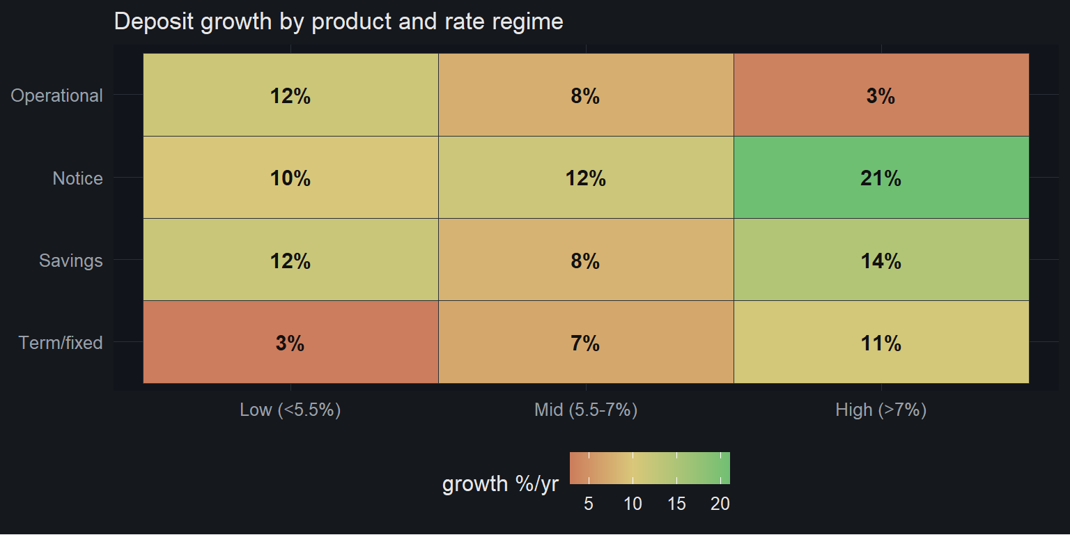
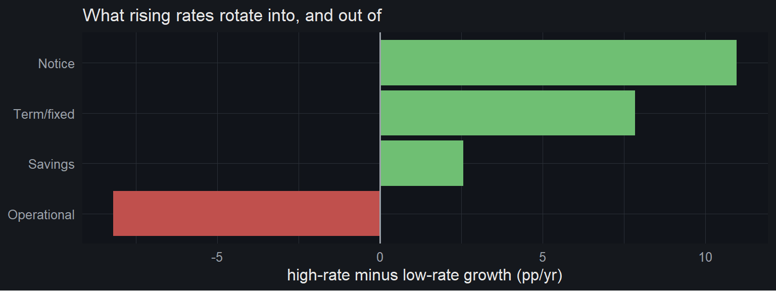
The regime map: annualised deposit growth by product and rate level, on the full SARB sector total. Operational balances fill up when rates are low and drain as they rise; term and notice do the reverse - the forward-looking rotation an ALCO can plan against.

Read the corners. In a low-rate regime, operational (current-account) balances grow ~11–12% a year while term deposits barely move (~3%). In a high-rate regime that inverts: term and notice pull money in hard (term ~11%, notice ~21%) while operational growth collapses to ~3%. This is flight-to-yield, and for an ALCO it is a planning map: as rates rise, expect your own operational book to stall and your term and notice books to swell - and budget the funding-cost and duration consequences before they arrive.

The rotation signal in one view: growth in a high-rate regime minus growth in a low-rate regime, per product. Positive bars are what rising rates rotate money into; negative bars are what they rotate out of.

The competition state and bank-level flows

The natural next question - can the competition state flag when deposits leave NGFB specifically - has a negative answer worth stating. Coupling the state to NGFB’s net flow, even with the correct sector denominator and tested per category, gives correlations indistinguishable from zero (full-state vs net flow ≈ −0.01; the largest per-category figure is savings at −0.18, still weak; the residual, level-stripped state likewise ≈ 0).

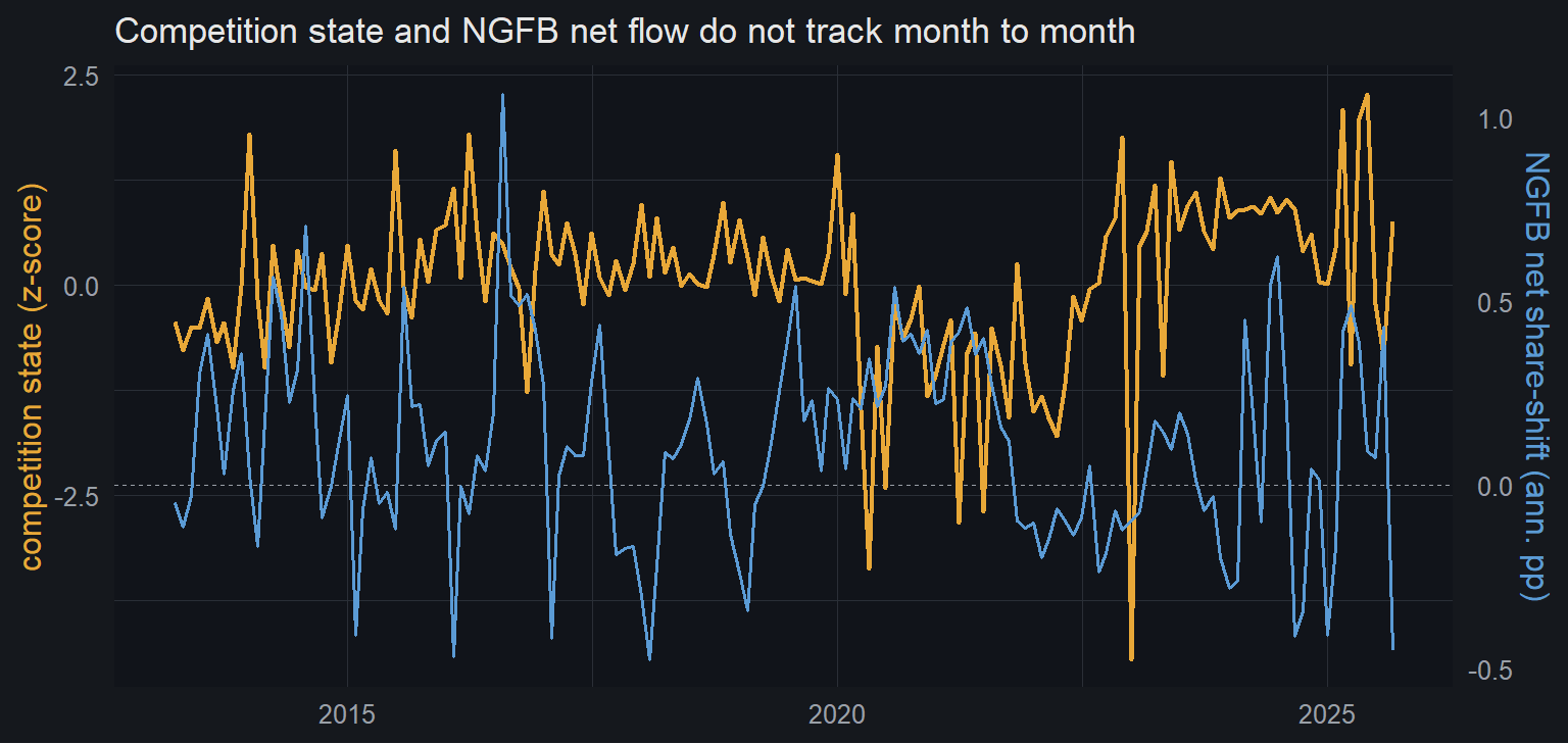
The competition state (gold) and NGFB’s net flow (blue, 6-month smoothed). They do not track month to month - the relationship is low-frequency and lives in the regime map above, not in contemporaneous co-movement. Shown so the reader sees the null directly.

This is not a failure of the model but a fact about the data - and partly a property of the synthetic-bank construction itself. NGFB’s net flow here is reconstructed as its canonical product mix riding the industry category paths, so by design it moves almost exactly with the sector; its only idiosyncratic component is the small compositional tilt, which is swamped by sector-wide variation. Competition therefore shows up as product rotation (the regime map), not as monthly bank-level wins and losses, and BA900’s net flows cannot see a silent run regardless.

📎

The null is partly about NGFB, not just about deposits

For a real bank the same test could come out differently. A real institution has genuine bank-specific flow - its own pricing, a branch-network change, a competitor targeting its base - that can diverge from the sector in ways NGFB's composition-weighted shadow cannot. So the competition state could correlate with bank-level deposit wins and losses for an actual bank, where for our synthetic one it cannot. The clean reading: from public BA900 aggregates, competition is identifiable through rotation between products, not through bank-level net inflows and outflows - but that boundary is set as much by the synthetic construction and the data's net aggregation as by deposit behaviour itself.

📎

What customer-level data would unlock

The deeper limit is that BA900 records net balances: a month where money quietly leaves while new money arrives nets to zero and is invisible. A bank with access to its own customer-level data - account counts and individual balances traced over time - observes gross flows: accounts opening, closing, and migrating. With that, the competition state could be correlated against true bank-level inflows and outflows, not just product rotation, and a silent run (the case Post 4's liquidity buffer is built to withstand) would become directly detectable rather than structurally hidden. The model is the same; the data resolution is what changes what it can see.

What this gives an ALCO that a flat beta does not

A constant deposit beta says nothing about where money sits - it treats the book as a fixed lump that reprices uniformly. The regime map says: at this rate level, expect this much migration out of operational and into term/notice, inside your own bank. That changes funding-cost projections (term is dearer than operational), liquidity planning (notice carries a withdrawal lag), and the duration of the book (term is longer). It is the difference between reacting to deposit migration and budgeting for it a regime ahead.

📎

Two honest limits on the map

It is a regime-level, low-frequency signal, not a monthly predictor. The contrast between rate regimes is strong, but the month-to-month correlation between the rate level and category growth is near zero, because deposit rotation responds with long, variable lags. Plan with it over the cycle, not the quarter.

It is net, not gross. The decomposition uses the published sector total (the six banks we model are ~95% of it). It cleanly shows which products gain or lose ground per regime - but a silent outflow masked by new money inside a single product-month is invisible.

The model behind the map

The regime map and the rate-risk number both come from one model: a single latent state, competitive search intensity $s_t$, driving both the price depositors are offered and the speed at which balances move. The intuition is one story - when depositors shop hard, banks must pass more of the rate move through (beta rises) and balances rotate faster - so one state sits behind both. The state is anchored to the rate level, with a small residual left for the filter:

$$ s_t = g(\text{repo}_t) + z_t, \qquad z_t = \rho\, z_{t-1} + \eta_t $$

where $g(\cdot)$ is the standardised repo level - a continuous regressor, not a discrete regime indicator - and $z_t$ is the persistent residual. The state loads onto two observation equations, pricing and flows:

$$ \Delta r^{\text{dep}}_{c,t} = \big(\beta_c + \lambda^\beta_c\, s_t\big)\,\Delta\text{repo}_t + \varepsilon^\beta_{c,t} $$$$ \Delta \log B_{c,t} = \mu_c + \big(\delta_c + \lambda^\delta_c\, s_t\big)\,\text{gap}_{c,t} + \varepsilon^\delta_{c,t} $$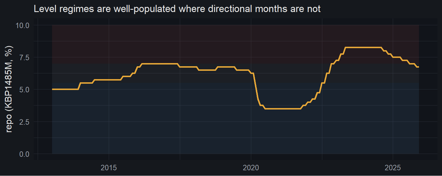

📎

Continuous, not regime-switching - and where it sits in the literature

There are no low/mid/high regimes in the model. Pass-through bends smoothly with the standardised level through $\beta_c + \lambda^\beta_c s_t$; the bands in the regime map are a reading aid for the output, not model structure. This is a level-anchored variant of Brigida's random-walk time-varying beta [@brigida2025], who is explicit that he uses a CUSUM test rather than a Chow/Quandt break test [@browndurbinevans1975; @chow1960] because coefficients drift smoothly rather than jump. Anchoring that drift to an observable driver - the rate level - rather than letting it random-walk freely is what makes it identify on South Africa's flat path, and it applies the continuous rate-dependence of [@dallasfed2023] to a shared pricing-and-flow state. The deposit-franchise premise throughout is [@drechsler2021].

The realised repo path, shaded by level band. The bands are a reading aid - they show the level has ample variation to estimate on, where the directional-change count is threadbare. The model sees the continuous level, not three bins.

Does each piece of the model earn its place?

Add the parts one at a time and watch the likelihood. On the real panel - 156 months, six rate cells, three flow cells - the gains stack cleanly.

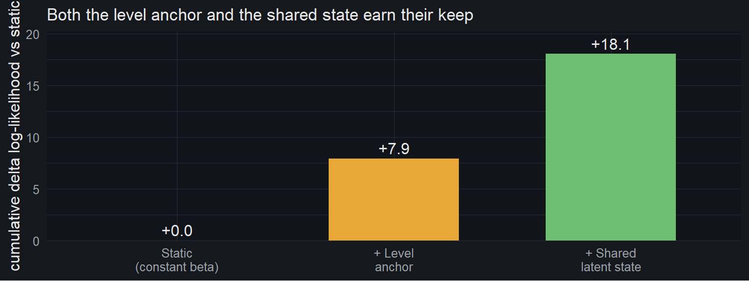
Log-likelihood gain over a constant-beta model. The level anchor adds 7.9 nats; the shared latent residual adds a further 10.1. Both earn their place.

The shared state is genuinely shared: decoupling it into two independent per-channel states improves the fit by essentially nothing,

$$ \text{LR} = 2\big(\ell_{\text{decoupled}} - \ell_{\text{coupled}}\big) \approx 0 \;<\; \chi^2_{3,\,0.95} = 7.82, $$

so one latent residual does the work in both channels - the “one driver” reading, identified rather than assumed. The honest caveat: the correlation between the two channels’ one-step innovations is only ~0.05, so the coupling is favoured by the likelihood but carried mostly by the level anchor.

What the pass-through looks like

The contemporaneous response of each cell’s deposit rate to a repo move orders exactly as deposit-franchise theory predicts.

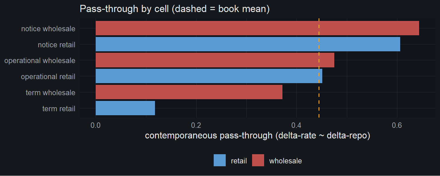
Contemporaneous pass-through by cell. Notice prices hardest (~0.6), term-retail is the stickiest book (0.12), wholesale beats retail within every category. This is the franchise, quantified.

Notice money is the most rate-sensitive - it reprices hardest because it is shopped hardest. Term-retail is the stickiest book at 0.12 - locked, barely following repo within the month, which is what makes it valuable franchise funding. Wholesale beats retail within every category. (These are one-month contemporaneous slopes, book-aggregate ~0.44; the long-run cumulative pass-through is higher.) The level-sensitivity loadings $\lambda^\beta_c$ are largest in the wholesale and notice books - where rate-sophisticated money lives - but modest in magnitude, which foreshadows the size of the rate-risk number.

The rate-risk number: what a flat beta costs you

The second deliverable. The level-dependence barely matters over one month - a constant beta tracks next month’s deposit cost about as well as anything. It matters over a cycle, and the place it shows up is the bank’s economic value of equity and its sensitivity to a rate shock. A bank assuming a flat beta computes one deposit duration; a bank that knows beta bends with the level computes another. The gap is a mismeasured risk position - invisible on bank balance sheets until 2023 made it expensive.

We run the standard ALCO instrument: an instantaneous parallel ±200bp shock, held, and compute the change in the present value of the franchise margin two ways - flat-beta and level-anchored - on NGFB’s canonical book. The discount curve is a synthetic ZAR curve (repo plus a fixed term-premium slope; the real swap curve is a Post 3 input), but it cancels: both legs use the identical curve and agree exactly at the current level, so only the beta treatment moves the numbers.

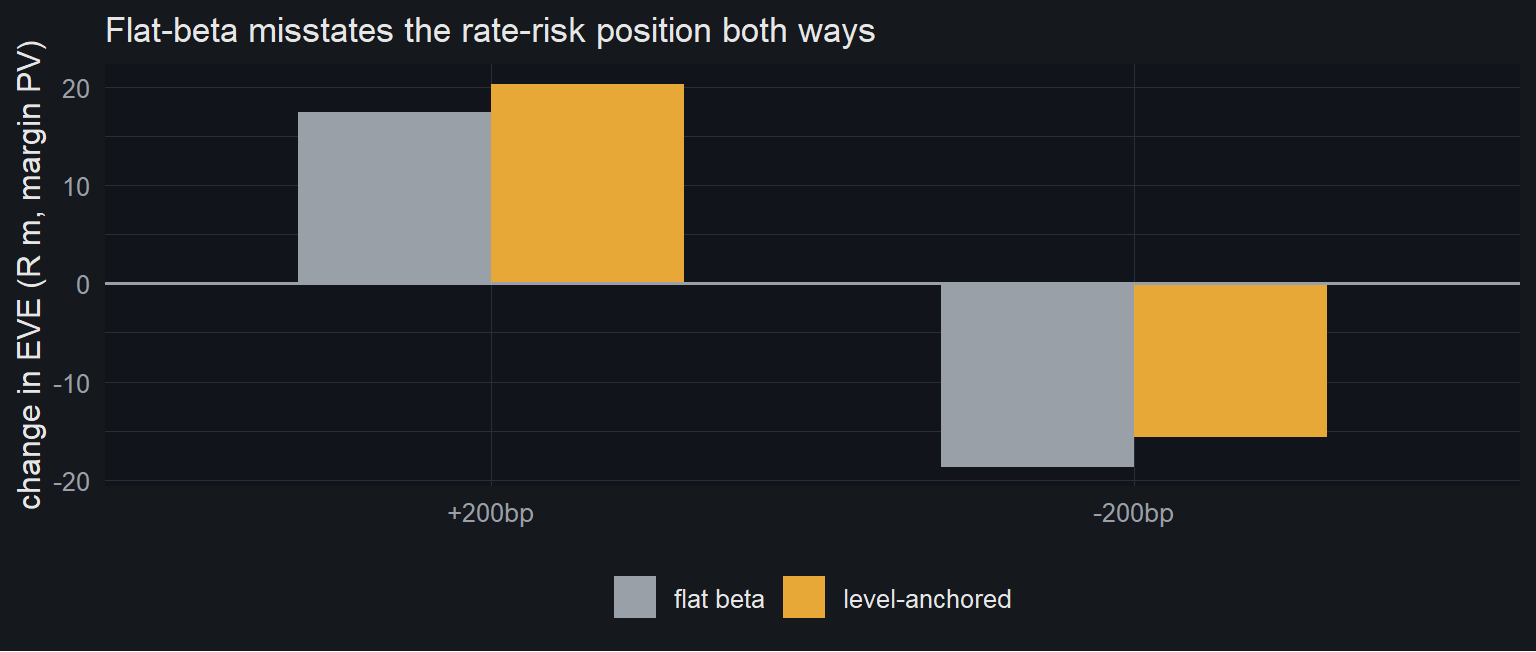
Change in EVE under plus/minus 200bp, flat-beta versus level-anchored, on NGFB’s canonical book. The model says the franchise gains more in a hike and loses less in a cut than the constant-beta assumption implies - the gap is the mismeasured risk.

The mismeasurement - the level-anchored ΔEVE minus the flat ΔEVE - is +31 bps of the deposit base on a +200bp shock and +34 bps on −200bp: a constant-beta bank misjudges how much its deposit value moves under a standard shock by roughly a third of a percent of the whole base, each way.

The asymmetry is the economically important part. The level-anchored franchise is less rate-sensitive on the downshock and more on the upshock - a signed convexity of about −2.3 bps. Because pass-through rises with the level, the deposit rate chases repo up more aggressively in a hike (compressing the margin gain) and lags it down in a cut (cushioning the margin loss). The franchise behaves like a book with an embedded option: more valuable when rates fall than a flat beta implies, less when they rise. The constant-beta bank is blind to exactly this curvature, and curvature is what hurts when the shock is large.

And the capital impact

The mismeasurement is a stock - a present value - not an annual flow, so the honest conversion is to capital, not to recurring ROE. Against core capital (deposits ~62% of assets, CET1 ~11.5%, RWA density ~0.55), the EVE error is ~3.1% of CET1 on +200bp and ~3.3% on −200bp: a flat-beta bank misstates economic equity by roughly a thirtieth of core capital under a standard shock, in a direction it cannot see. Annualised over the book’s ~1.6-year average life it is a ~109 bps ROE drag in a stress year - but that flow restatement is the softer figure (it annualises a stock) and is reported as secondary to the capital number.

Behavioural duration, two ways

The EVE depends on how long deposits behaviourally last, so the duration measurement matters. We measure it two independent ways and the headline survives both.

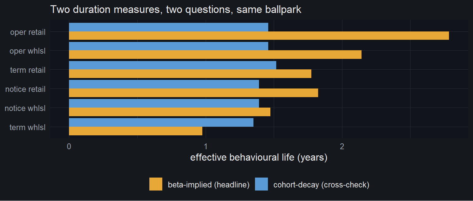
Behavioural life by cell, two methods. Beta-implied (gold, the headline) asks how the rate reprices; cohort-decay (blue, the cross-check) asks how an injection of money runs off. Different questions, different orderings, same ballpark - and the EVE survives either.

The primary measure is beta-implied effective duration (the BCBS IRRBB replicating-portfolio logic (Basel Committee on Banking Supervision 2016)): the repricing fraction of each category floats with the market, the core fraction is stable funding capped at the regulatory average maturity. It gives operational ~2.5y, notice ~1.6y, term ~1.4y, franchise ordering intact. The cross-check is a cohort/shock-decay impulse response - inject a unit of balance, trace how much survives at each month, cap at four years - asking a different question (injection survival, not repricing speed) and giving a different ordering but the same EVE headline within a third (~26 bps versus ~31–34 bps).

📎

Why rate-sensitivity, not balance-decay, carries the duration

An unobserved-components decomposition of each balance into a permanent (random-walk) and a transitory (stationary) component settles which measure to trust. The transitory persistence is near zero for operational, notice and term - a shock to the level of these balances does not revert; it is permanent. SA NMD balances are, empirically, random walks with drift [@kanglandsberg2022]. That is why balance-decay carries almost no duration information at the aggregate level, and why the regulatory standard measures rate sensitivity rather than runoff speed. The cohort method recovers a usable decay only because it asks about an injection's survival, not the level's reversion.

The mathematics, in full

State-space form

The latent state is the scalar residual $z_t$ on top of the observable level anchor $g_t = (\text{repo}_t - \bar r)/\sigma_r$, so $s_t = g_t + z_t$ with transition $z_t = \rho z_{t-1} + \eta_t$, $\eta_t \sim \mathcal N(0,\sigma_\eta^2)$. Each pricing cell observes a deposit-rate change with pass-through affine in the state; each flow cell a log-balance change responding to the lagged spread:

$$ \Delta r^{\text{dep}}_{c,t} = \beta_c\Delta\text{repo}_t + \lambda^\beta_c g_t\Delta\text{repo}_t + \lambda^\beta_c z_t\Delta\text{repo}_t + \varepsilon^\beta_{c,t} $$$$ \Delta \log B_{c,t} = \mu_c + \delta_c\,\text{gap}_{c,t} + \lambda^\delta_c g_t\,\text{gap}_{c,t} + \lambda^\delta_c z_t\,\text{gap}_{c,t} + \varepsilon^\delta_{c,t} $$

Stacking present rows gives a linear-Gaussian system with one-dimensional state, $y_t = d_t + Z_t z_t + \epsilon_t$, $\epsilon_t \sim \mathcal N(0,H_t)$. The level part lives in the known intercept $d_t$; the loading $Z_t$ carries $\lambda$ times the regressor. The sample is ragged (rates from 2013, volumes from 2008), handled by dropping absent rows.

Kalman recursion

Since $g_t$ is known, the filter tracks only the scalar $z_t$. With $z_0 \sim \mathcal N(0, \sigma_\eta^2/(1-\rho^2))$:

$$ a_{t|t-1} = \rho a_{t-1}, \quad P_{t|t-1} = \rho^2 P_{t-1} + \sigma_\eta^2 $$$$ v_t = y_t - (d_t + Z_t a_{t|t-1}), \quad F_t = Z_t P_{t|t-1} Z_t^\top + H_t $$$$ K_t = P_{t|t-1} Z_t^\top F_t^{-1}, \quad a_t = a_{t|t-1} + K_t v_t, \quad P_t = (1 - K_t Z_t)P_{t|t-1} $$

The prediction-error decomposition gives the log-likelihood, $\ell(\theta) = -\tfrac12 \sum_t [ n_t\log 2\pi + \log|F_t| + v_t^\top F_t^{-1} v_t ]$.

Concentrating out the statics

The free parameters are $\theta=\{\rho,\sigma_\eta,\lambda^\beta_\cdot,\lambda^\delta_\cdot\}$. The static terms $\{\beta_c,\delta_c,\mu_c\}$ and noise variances are concentrated out - for any $\theta$ they are the OLS optimum on the level-and-latent-adjusted observation. Scale is fixed by standardising $g_t$ to unit variance. Estimation is L-BFGS-B over $\{\text{logit}\rho,\log\sigma_\eta,\lambda\}$ with box bounds, multi-started to avoid the degenerate escape where $\sigma_\eta\to\infty$ and loadings collapse.

Where the EVE numbers come from, exactly

1. Margin. For cell $c$ at market level $R$, monthly margin on balance $B_c$ is $m_c(R) = \tfrac{R - r^{\text{dep}}_c(R)}{1200} B_c$.

2. Pass-through. $r^{\text{dep}}_c(R) = r^{\text{dep}}_{c,0} + b^{\text{eff}}_c(R)(R-R_0)$, flat uses $b^{\text{eff}}_c=\beta_c$, level-anchored uses $b^{\text{eff}}_c = \beta_c + \lambda^\beta_c(g(R)-g(R_0))$. Both equal $\beta_c$ at $R=R_0$, so the EVE bases match and only the shock response differs.

3. Runoff. Balances amortise at $\alpha_c = 1/L_c$; survivor at month $t$ is $B_c(1-\alpha_c)^{t-1}$.

4. Discounting. Synthetic ZAR curve $DF(R,t)=(1+\tfrac1{12}[R+\tau t/12]/100)^{-t}$; cancels in the difference.

5. EVE and mismeasurement.

$$ \mathrm{EVE}_p(R) = \sum_c \sum_{t=1}^{240} \frac{R - r^{\text{dep},p}_c(R)}{1200} B_c (1-\alpha_c)^{t-1} DF(R,t) $$$$ \Delta\mathrm{EVE}_p = \mathrm{EVE}_p(R_0+\Delta) - \mathrm{EVE}_p(R_0), \quad \text{Mismeas} = \Delta\mathrm{EVE}_{\text{level}} - \Delta\mathrm{EVE}_{\text{flat}} $$

6. Duration $L_c$. Beta-implied: $L_c = \beta_c\cdot 1 + (1-\beta_c)\bar L_c$, $\bar L_c$ the BCBS core cap. Cohort cross-check: AR(2) on the drift-removed log balance gives retention $r_k$; core $=r_{48}$, non-core amortises on $r_k$.

7. EVE error to capital. With deposits/assets 0.62, CET1 11.5%, RWA density 0.55:

$$ \frac{\Delta\mathrm{EVE}}{\mathrm{CET1}} = \frac{0.00313 \times 0.62}{0.115 \times 0.55} = \frac{0.00194}{0.06325} = 3.07\% \text{ of CET1}. $$

Defining NGFB: the canonical composition draw

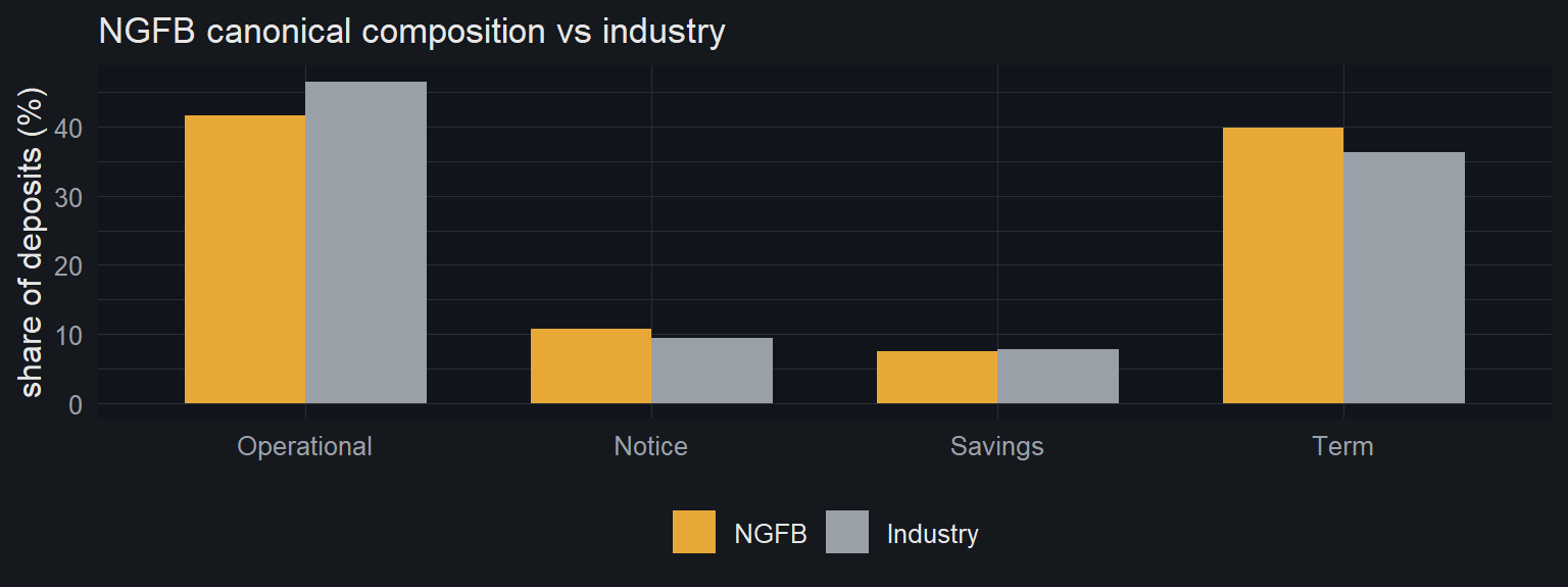
The synthetic bank’s product mix is fixed as a single draw from a hierarchical model of deposit composition across the six majors. Each bank’s share vector is mapped to additive-log-ratio space and modelled as multivariate normal, $x_b \sim \mathcal N(\mu,\Sigma)$; the hyperparameters $\mu,\Sigma$ are the only published objects (individual mixes integrated out, satisfying the aggregation rule). NGFB is a posterior-predictive draw $x^\star \sim \mathcal N(\mu,\Sigma)$, truncated to within one standard deviation (Mahalanobis $\le 1$) so it is idiosyncratic but representative, not a tail bank, then mapped back through the softmax. The canonical draw is 42% operational, 11% notice, 7.5% savings, 40% term - modestly term- and notice-tilted versus the industry. The draw is seeded and fixed: NGFB’s identity for the whole series, and every balance-weighted figure uses it.

NGFB’s canonical composition (a truncated hierarchical draw) against the industry average. Modestly term- and notice-tilted - a credible franchise-funded bank, idiosyncratic but not a tail.

What didn’t work

Key findings from things that came out inconsistent or counter-intuitive, with reasons.

Competition does not couple to deposit flows at monthly frequency. The competition state is, by construction, mostly the rate level. Coupling it to NGFB’s net flow - after fixing the denominator to the full sector and testing every category - gives correlations indistinguishable from zero (the residual, level-stripped state likewise). The rate-cycle-to-rotation relationship is real but low-frequency and lagged: it shows up as the strong regime contrast above and washes out month to month. A monthly overlay was the wrong instrument for a slow relationship; the regime map is the right one.
The missing 5% of the sector is not a hidden outflow. We model six banks (~95% of sector deposits); the rest sit in the gap to the BA900 sector total. A reasonable worry was that deposits were quietly leaving the majors for the digital banks unseen. The data say the opposite - the six-bank share rose from 92% to 95%, so the majors gained ground against the smaller banks. We use the published sector total as the denominator regardless, as the correct reference.
Balance-decay duration measured naively is meaningless on these series. A simple AR(1) on the balances gives a behavioural life of about six weeks - absurd. The reason is structural: the UC decomposition shows the balances are random-walk-permanent, so a detrended AR latches onto sub-monthly noise. Balance-decay does not encode duration for SA NMDs; rate-sensitivity does. A clean confirmation of why the regulatory replicating-portfolio standard exists.
The “competition intensifies in cuts” conjecture is weak in pricing and absent in flows. The convexity story suggested cutting cycles should see extra competitive pass-through. Tested directly, the asymmetry is correctly signed but significant in only one of six pricing cells, and absent in the runoff channel. Forced into the EVE it offsets rather than amplifies. Carried as a labelled sensitivity, not a result.
The shared latent state buys fit, not repricing. It earns +10.1 nats but the channel-innovation correlation is ~0.05 and it adds nothing to one-month-ahead repricing. Its value is in the duration/EVE picture and the flow coupling, which is why the post measures value through EVE and the regime map, not a repricing bridge.
Inherited data limits. BA930 rates are sector-aggregate (a feature under the aggregation rule) and start in 2013; no published savings rate (savings is flow-only); BA900 volumes reach to 2008, which helps anchor the state where the rate channel cannot see.

📎

Provenance and reproducibility

Every number is DERIVED from the named SARB series via the pipeline or ASSUMED as a stated balance-sheet input. DERIVED: the pass-through betas, the likelihood decomposition (+5.9, +11.9 nats), the LR (~0), the regime-map growth rates, the EVE mismeasurement (31/34 bps), the durations, the UC permanence result, and NGFB's composition draw. ASSUMED: the BCBS core caps, the 240-month horizon, the synthetic term-premium slope (which cancels), and the representative balance sheet (deposits/assets 0.62, CET1 11.5%, RWA density 0.55). The discount curve is synthetic and stated as such; the EVE headline is a difference on the identical curve. The regime map, rotation tilt and repo-path figures compute live from the committed SARB data.

Basel Committee on Banking Supervision. 2016. Interest Rate Risk in the Banking Book. Standards No. d368. Bank for International Settlements. https://www.bis.org/bcbs/publ/d368.htm.

Brigida, Matt. 2025. Time-Varying Volatility of Bank Betas. arXiv preprint arXiv:2510.07671. https://arxiv.org/abs/2510.07671.

Brigida, Matt, and Kathleen Brigida. 2025. “Time-Variation in Bank Income and Expense Betas.” Managerial Finance 51 (2): 206–15.

Brown, Robert L., James Durbin, and James M. Evans. 1975. “Techniques for Testing the Constancy of Regression Relationships over Time.” Journal of the Royal Statistical Society, Series B 37 (2): 149–92.

Chow, Gregory C. 1960. “Tests of Equality Between Sets of Coefficients in Two Linear Regressions.” Econometrica 28 (3): 591–605.

Drechsler, Itamar, Alexi Savov, and Philipp Schnabl. 2017. “The Deposits Channel of Monetary Policy.” Quarterly Journal of Economics 132 (4): 1819–76. https://doi.org/10.1093/qje/qjx019.

Drechsler, Itamar, Alexi Savov, and Philipp Schnabl. 2021. “Banking on Deposits: Maturity Transformation Without Interest Rate Risk.” Journal of Finance 76 (3): 1091–143. https://doi.org/10.1111/jofi.13013.

Greenwald, Emily, Sam Schulhofer-Wohl, and Joshua Younger. 2023. Deposit Convexity, Monetary Policy and Financial Stability. Working Paper No. 2315. Federal Reserve Bank of Dallas. https://www.dallasfed.org/research/papers/2023/wp2315.

Kang-Landsberg, Alena, and Matthew Plosser. 2022. “How Do Deposit Rates Respond to Monetary Policy?” Federal Reserve Bank of New York Liberty Street Economics.