Forecasting South African Government Bond Yields
The question
This is going to be a longer-than-average post for what looks, on the surface, like a small empirical question. The answer turns out to be structurally clean and slightly counter-intuitive, which is reason enough to write it down carefully. Here’s the framing.
For a multi-tenor yield curve, two natural modelling philosophies exist:
- Direct forecasting: build a separate model per tenor and per horizon, predicting that tenor’s future yield from its own lags (and possibly the other tenors’ lags). The model has full flexibility per cell.
- Factor decomposition: parameterise the entire curve at each date as a small number of factors (level, slope, curvature in the Nelson-Siegel framework), forecast the factors, then reconstruct each tenor’s forecast from the predicted factors. The model imposes cross-sectional consistency.
Both have well-known strengths. Direct models can fit tenor-idiosyncratic dynamics that factor decompositions paper over. Factor models give curve-consistent forecasts and reduce the parameter count — at long horizons, where signal-to-noise ratios are unfavourable, that parsimony usually wins. Where exactly does the trade-off sit on monthly South African government data?
This post answers that empirically. Five direct-modelling approaches — AR(1), Ridge regression, Elastic Net, a small neural network, and LightGBM — race against two factor approaches — Dynamic Nelson-Siegel with AR(1) per factor (DNS) and DNS with arbitrage-free bias correction (AFNS) — across four SARB government bond maturity buckets (0-3Y, 3-5Y, 5-10Y, 10-15Y) and six horizons (1, 3, 6, 12, 24, 60 months). Naive (random walk) is the benchmark. Macros are deliberately excluded so this post is a clean comparison of model families; they’ll get their own post in a follow-up.
Data and setup
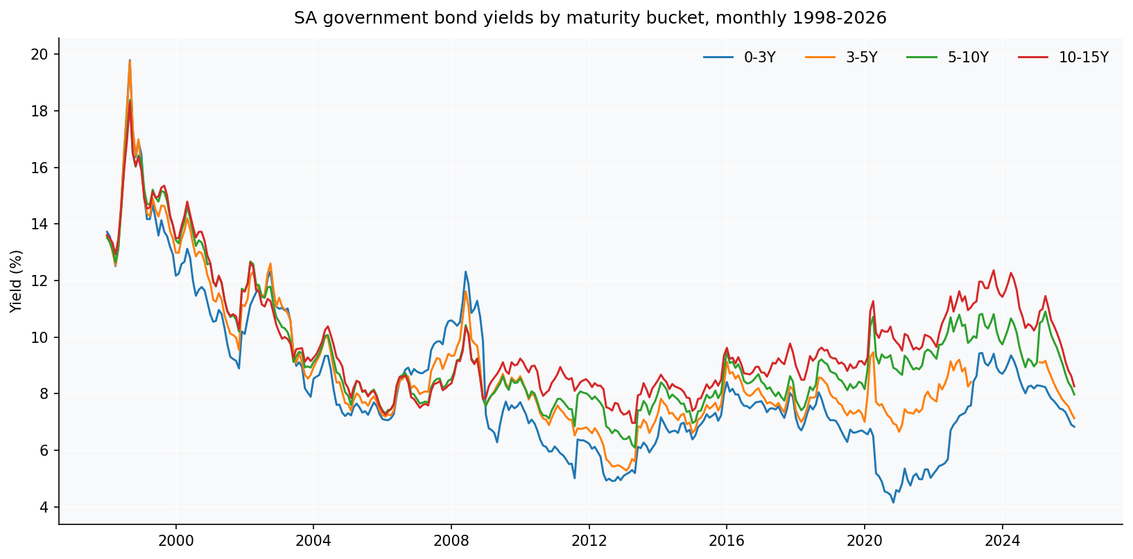
Yields
Four South African government nominal bond yield series from the SARB Quarterly Bulletin, monthly from January 1998 through February 2026. These are maturity-range buckets, not specific tenors:
| SARB code | Description | Bucket midpoint |
|---|---|---|
KBP2000M | Government bonds, 0-3 years nominal yield | 1.5 years |
KBP2001M | Government bonds, 3-5 years nominal yield | 4.0 years |
KBP2002M | Government bonds, 5-10 years nominal yield | 7.5 years |
KBP2003M | Government bonds, 10-15 years nominal yield | 12.5 years |
Each series is the average yield on currently-traded government bonds whose remaining maturity falls in the corresponding bucket. There is no separate publication of specific-tenor government bond yields (no “3M government bond yield”, no “10Y on-the-run yield”) in the QB monthly tables — bucket aggregates are the deepest cross-sectional granularity SARB provides at monthly frequency. One important caveat about the 3-5Y bucket — see the “data caveat” subsection below.
A data caveat: the 3-5Y bucket gap
One important data hygiene note. The 3-5Y yield series (KBP2001M)
has 23 consecutive months of missing data, from March 2023 to
January 2025. This is in the SARB source itself, not introduced by
the data pipeline. The cause is documented on SARB’s Current Market
Rates page, footnote 6:
The R2023 government bond matured on 28 February 2023 and is therefore no longer published
The R2023 government bond, in its final months of trading, was a significant component of the 3-5 year maturity bucket. Then it did what all bonds eventually do; it matured, inconsiderately, leaving a two-year hole in the data and a small lesson about depending on a single benchmark. When R2023 matured at end-February 2023, the 3-5Y bucket was thinly populated. The next benchmark government bond (R186, maturing 2026) was right at the 3-year boundary and migrated into the 0-3Y bucket during this period, leaving the 3-5Y bucket empty until new short-dated bonds were issued. SARB resumed publishing the 3-5Y series from February 2025.
Alternative sources considered. Independent SA fixed-income data providers (notably rbond.co.za, curated from JSE YieldX since 2018) publish daily yields for specific R-bonds. But constructing a bucket-equivalent average yield from those would require choosing how to weight bonds — a methodology decision that differs from SARB’s internal construction.
Choice made. The gap is left unfilled. Dropping affected rows is more honest than injecting synthetic continuity. The impact is small and quantifiable: 2-4 forecasts dropped per cell for the 3-5Y tenor’s evaluation, leaving each cell with 27-35 valid evaluation points; about 23 training rows dropped during late walk-forward steps for the other tenors that use the 3-5Y lag as a feature. Statistical power on the 3-5Y bucket is slightly reduced.
What the yield data looks like statistically
Three statistical facts that constrain what any forecasting model can hope to achieve. These aren’t decoration — they predetermine which models can succeed and which are dead on arrival.
Augmented Dickey-Fuller tests and AR(1) persistence by tenor. The “Stationary” columns mark ✓ when the ADF null of a unit root is rejected at p < 0.05.
| Bucket | ADF (levels) | p-value | Stationary? | ADF (Δ) | p-value | Stationary | AR(1) φ |
|---|---|---|---|---|---|---|---|
| 0-3Y | -2.57 | 0.100 | ✗ | -13.34 | 6.00e-25 | ✓ | 0.9801 |
| 3-5Y | -2.15 | 0.224 | ✗ | -12.47 | 3.31e-23 | ✓ | 0.9788 |
| 5-10Y | -2.17 | 0.217 | ✗ | -13.21 | 1.04e-24 | ✓ | 0.9789 |
| 10-15Y | -2.16 | 0.220 | ✗ | -9.59 | 2.07e-16 | ✓ | 0.9805 |
The interpretation is unusually clean. Yields are I(1) — first differences are stationary, levels are not. AR(1) persistence is 0.979-0.981 across every bucket. That gives a theoretical RMSSE lower bound (relative to random walk) of $\sqrt{(1+\phi^h)/2}$ — about 0.99 at h=1, 0.93 at h=12, and 0.78 at h=60.
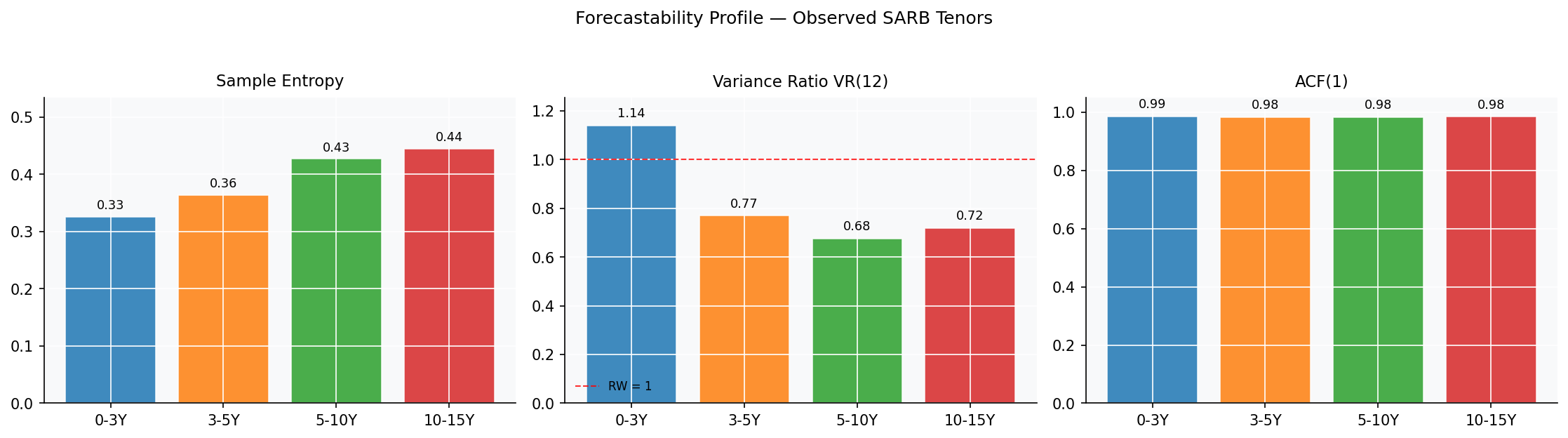
Forecastability metrics in one sentence each.
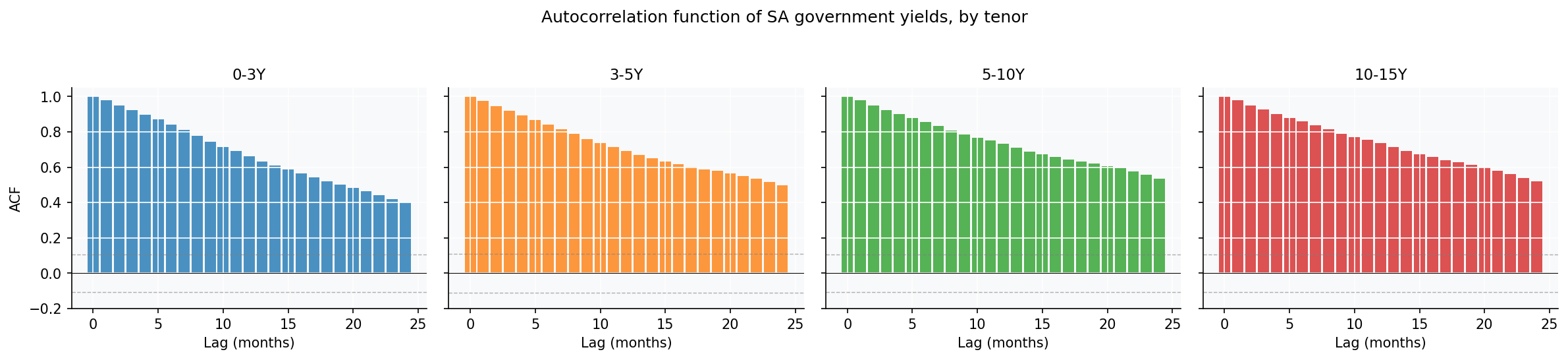
- ACF(1) is the lag-1 autocorrelation of yields. Near 1 means “today is an excellent predictor of next month”.
- Variance Ratio VR(12) is $\text{Var}(y_t - y_{t-12}) \,/\, [12 \cdot \text{Var}(y_t - y_{t-1})]$. For a pure random walk it equals 1; values below 1 signal mean reversion at the 12-month horizon, values above 1 signal momentum.
- Sample Entropy measures the unpredictability of short-pattern recurrence. Lower values mean more deterministic structure; higher values mean more white-noise-like.
All four buckets live in “near-random-walk” territory by every metric. There’s no hidden tractable structure waiting to be exploited.
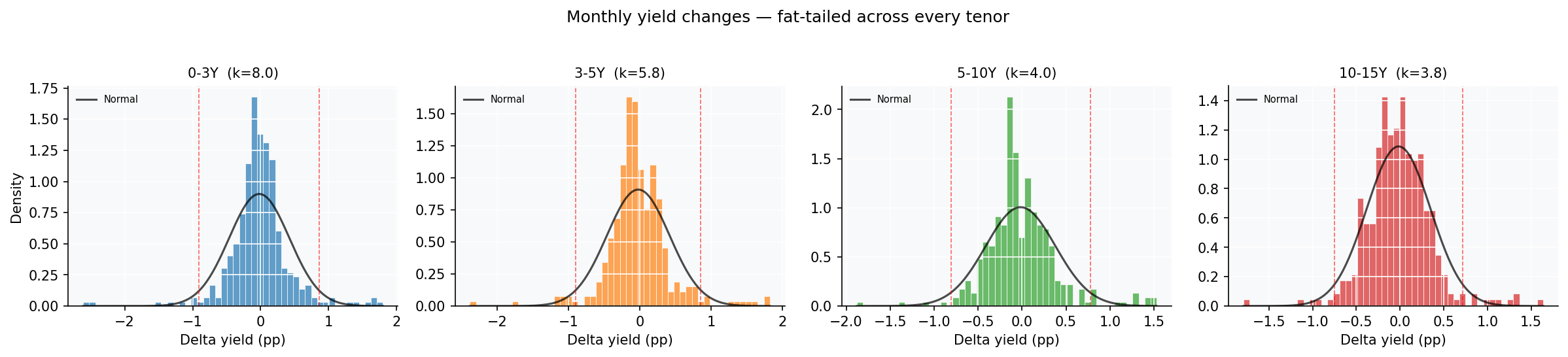
Jarque-Bera rejects normality at p<0.001 for every tenor, with kurtosis 4-11 against the Gaussian 3. The 0-3Y bucket has noticeable negative skew. Bottom line: yields are persistent, non-stationary in levels, and have fat-tailed innovations. Any Gaussian-error parametric forecaster will understate tail risk.
Evaluation protocol
- Initial training window: 96 months (8 years).
- Walk-forward step: 6 months.
- Forecast horizons: h = 1, 3, 6, 12, 24, 60 months.
- h-step direct forecasting: at each walk-forward step $T$, models are trained on pairs $(X_t, y_{t+h-1})$ where both are observable at time T. Features at row $t$ depend only on $y_{t-1}$ and earlier. No future value of the target is used as a feature.
- Metrics: RMSE (pp), RMSSE (ratio to naive on same WFV set), DA (proportion correct sign of change from $y_{t-1}$ to $y_{t+h-1}$).
Level, slope, curvature — what DNS does
Three numbers to describe an entire yield curve. It is the kind of dimensionality reduction that makes a quant feel powerful right up until the forecasting starts.
The Nelson-Siegel decomposition (Nelson and Siegel 1987) writes the yield curve as
$$y_t(\tau) = \beta_{1t} + \beta_{2t}\,\frac{1-e^{-\lambda\tau}}{\lambda\tau} + \beta_{3t}\!\left[\frac{1-e^{-\lambda\tau}}{\lambda\tau} - e^{-\lambda\tau}\right]$$DNS forecasts the entire curve by treating the three factors as time series and reconstructing yields from forecasted factors. AFNS (Christensen et al. 2011) adds an arbitrage-free correction: a per-tenor constant bias $\hat\delta_\tau = \text{mean}(y_\tau - \hat y^{\mathrm{DNS}}_\tau)$ estimated on training data and added to the DNS forecast.
But which model forecasts the factors? The original Diebold-Li recipe (Diebold and Li 2006) uses an AR(1) per factor — three independent univariate models. The richer alternative is a VAR(p) on the three factors jointly, which captures cross-factor dependencies (the slope responding to level moves, the curvature catching up to slope, and so on). VAR is the textbook richer choice; AR(1) per factor is the parsimonious one. There is no a-priori reason to prefer either, so the tournament below tests four factor dynamics models head-to-head under identical evaluation protocol: random walk per factor (the no-information benchmark), AR(1) per factor (the Diebold-Li default), VAR(1) with eigenvalue clipping, and a Bayesian-style Ridge VAR with random-walk Minnesota prior. The headline DNS and AFNS results reported in subsequent sections use the AR(1) variant; the factor dynamics horse race in section “Which factor dynamics?” justifies that choice empirically.
Mathematical framework
For reference, here are the models in the tournament in their compact mathematical form. Same data goes into all of them; different inductive biases come out.
Naive (random walk). The benchmark.
$$\hat y_{t+h-1} \;=\; y_{t-1}$$AR(1) per tenor. With $\phi$ capped at 0.99 for stability.
$$y_{t+1} \;=\; c + \phi \, y_t + \varepsilon_t, \qquad \hat y_{t+h-1} = \mu + \phi^h\,(y_{t-1} - \mu), \quad \mu = \tfrac{c}{1-\phi}$$Ridge regression. L2 penalty; shrinks all coefficients smoothly.
$$\hat \beta_{\text{ridge}} \;=\; \arg\min_{\beta} \; \tfrac{1}{2n} \|y - X\beta\|_2^2 + \alpha\, \|\beta\|_2^2$$Lasso. Pure L1 penalty; drives coefficients to exactly zero.
$$\hat \beta_{\text{lasso}} \;=\; \arg\min_{\beta} \; \tfrac{1}{2n} \|y - X\beta\|_2^2 + \alpha\, \|\beta\|_1$$Elastic Net. L1 + L2 mix, controlled by $\rho \in [0,1]$.
$$\hat \beta_{\text{enet}} \;=\; \arg\min_{\beta} \; \tfrac{1}{2n} \|y - X\beta\|_2^2 + \alpha\!\left[\rho\,\|\beta\|_1 + \tfrac{1-\rho}{2}\,\|\beta\|_2^2\right]$$LightGBM. Additive ensemble of gradient-boosted trees; $\nu$ is the learning rate, $f_m$ the $m$th tree.
$$\hat y^{(M)} \;=\; \sum_{m=1}^{M} \nu\, f_m(\mathbf{x})$$Nelson-Siegel (DNS) with $\lambda = 0.25$ (curvature peak at $\tau^* \approx 3.3$ years, appropriate for the observed 1.5-12.5Y bucket midpoint spacing). Curve at each date parameterised by three factors:
$$y_t(\tau) \;=\; \beta_{1t} + \beta_{2t} \,\frac{1 - e^{-\lambda\tau}}{\lambda\tau} + \beta_{3t} \!\left[\frac{1 - e^{-\lambda\tau}}{\lambda\tau} - e^{-\lambda\tau}\right]$$Yield reconstruction from forecasted factors:
$$\hat y_{t+h-1}(\tau) \;=\; \hat\beta_{1,t+h-1}\, L_1(\tau) + \hat\beta_{2,t+h-1}\, L_2(\tau) + \hat\beta_{3,t+h-1}\, L_3(\tau)$$AFNS. DNS plus a per-tenor constant bias estimated on training data.
$$\hat y^{\text{AFNS}}_{t+h-1}(\tau) \;=\; \hat y^{\text{DNS}}_{t+h-1}(\tau) + \hat\delta_\tau, \qquad \hat\delta_\tau = \overline{\,y_\tau - \hat y^{\text{DNS}}_\tau\,}$$Factor dynamics. Eight choices for forecasting the three factors $f_t = (\beta_{1t}, \beta_{2t}, \beta_{3t})$ forward.
RW per factor: $f_{t+h} = f_t$.
AR(1) per factor: same as the direct AR(1) above, applied independently per factor.
VAR(1) with eigenvalue clip: if $\max|\text{eig}(A)| \ge 1$, scale $A$ to bring it to 0.99 and recompute $c$ so $\bar f_{\text{LR}}$ = sample mean.
$$f_{t+1} = c + A\, f_t + \varepsilon_t$$BVAR with RW prior (Ridge-VAR on changes). Predict $\Delta f$, shrink toward zero $\Leftrightarrow$ shrink toward random walk per factor:
$$\Delta f_{t+1} = c + A\, f_t + \varepsilon_t, \qquad \hat A = \arg\min \tfrac{1}{2n}\|\Delta F - F A\|_F^2 + \alpha\|A\|_F^2$$Lasso / Ridge / Elastic Net / LightGBM on factors. Per-factor direct $h$-step forecast of the factor change, using the rich 15-feature lag-only set computed on the factors themselves. Predicted change is added to the last observed factor level:
$$\hat f_{i,\, t+h-1} \;=\; f_{i,\, t-1} + \hat{g}_i(\mathbf{x}_{i,t})$$where $\hat g_i$ is the trained ML model for factor $i$.
The model tournament
A small zoo of models, all forecasting under the same h-step direct protocol, all on the same lag-only feature set (for the direct models). May the most parsimonious inductive bias win.
Six direct-forecasting models (one model per tenor and horizon):
- Naive (random walk): $\hat y_{t+h-1} = y_{t-1}$. Benchmark.
- AR(1) with constant per tenor, $\phi$ capped at 0.99.
- Ridge (alpha=5) on standardised lag-only features.
- Lasso (alpha=0.05) — pure L1, drops features to exactly zero.
- Elastic Net (alpha=1, l1_ratio=0.5) — L1+L2 mix.
- LightGBM (200 trees, depth 4, 15 leaves).
All five share the same ~17-feature lag-only set: own-tenor lags 1, 2, 3, 6, 12; cross-tenor lag-1 of the other four tenors; rolling mean and std at windows 3 and 12; first-difference lags ($\Delta_1$, $\Delta_{12}$); seasonal harmonics ($\sin$, $\cos$ of month).
Eight factor-decomposition models (one curve-wide model each). The structure is 4 factor-dynamics x 2 reconstruction choices:
7-10. DNS-RW / DNS-AR(1) / DNS-VAR / DNS-BVAR: extract level, slope, curvature; forecast each via random walk, AR(1) per factor with $\phi$ capped, VAR(1) with eigenvalue clipping, or Bayesian VAR with random-walk Minnesota prior; reconstruct yields from the factor forecasts.
11-14. AFNS-RW / AFNS-AR(1) / AFNS-VAR / AFNS-BVAR: the four DNS variants with per-tenor constant bias correction added.
The “headline” comparisons that follow use the AR(1) dynamics — DNS-AR(1) and AFNS-AR(1) — to keep the charts legible. A dedicated “Which factor dynamics?” section below works through the full comparison of all four dynamics models head-to-head.
Full scoreboard
Direct Lasso vs Direct Ridge — does L1 help on yields directly?
A natural side-question: on the direct yield models, does Lasso — with its hard zeros — actually beat Ridge, which only shrinks? Both fit the same lag-only feature set on the same training data with the same target. Only the regularisation differs.
Lasso wins the 5-10Y bucket at short-to-medium horizons (by 4-6%) and the 0-3Y bucket at long horizons (by 2-7%); Ridge wins the h=1 cells for the two shortest buckets (by 5-6%) and the 10-15Y bucket at h=60 (by 8%). Across all 24 cells it roughly washes out.
The interpretation: lag_1 is the dominant feature for yield forecasting, and both Ridge and Lasso keep it heavily weighted. The difference between them is only in how they handle the secondary features — cross-bucket lags, rolling stats. Lasso zeros the noisier ones; Ridge shrinks but retains them. On this data that distinction is second-order. In practice: use Lasso or Ridge interchangeably for direct yield forecasting; the regularisation choice barely moves the needle, and the horizon and bucket matter far more.
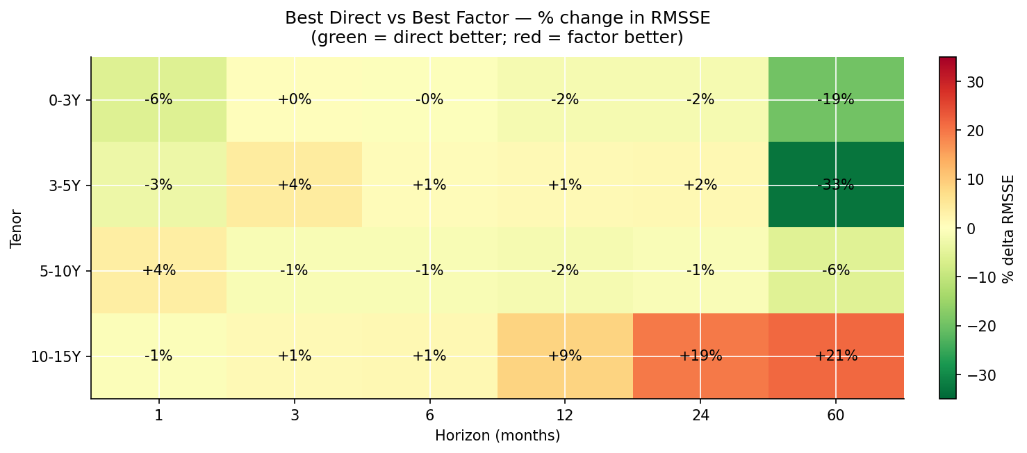
Direct vs factor — the head-to-head
The cleanest way to settle the central question is to compare the best direct model per cell against the best factor model per cell.
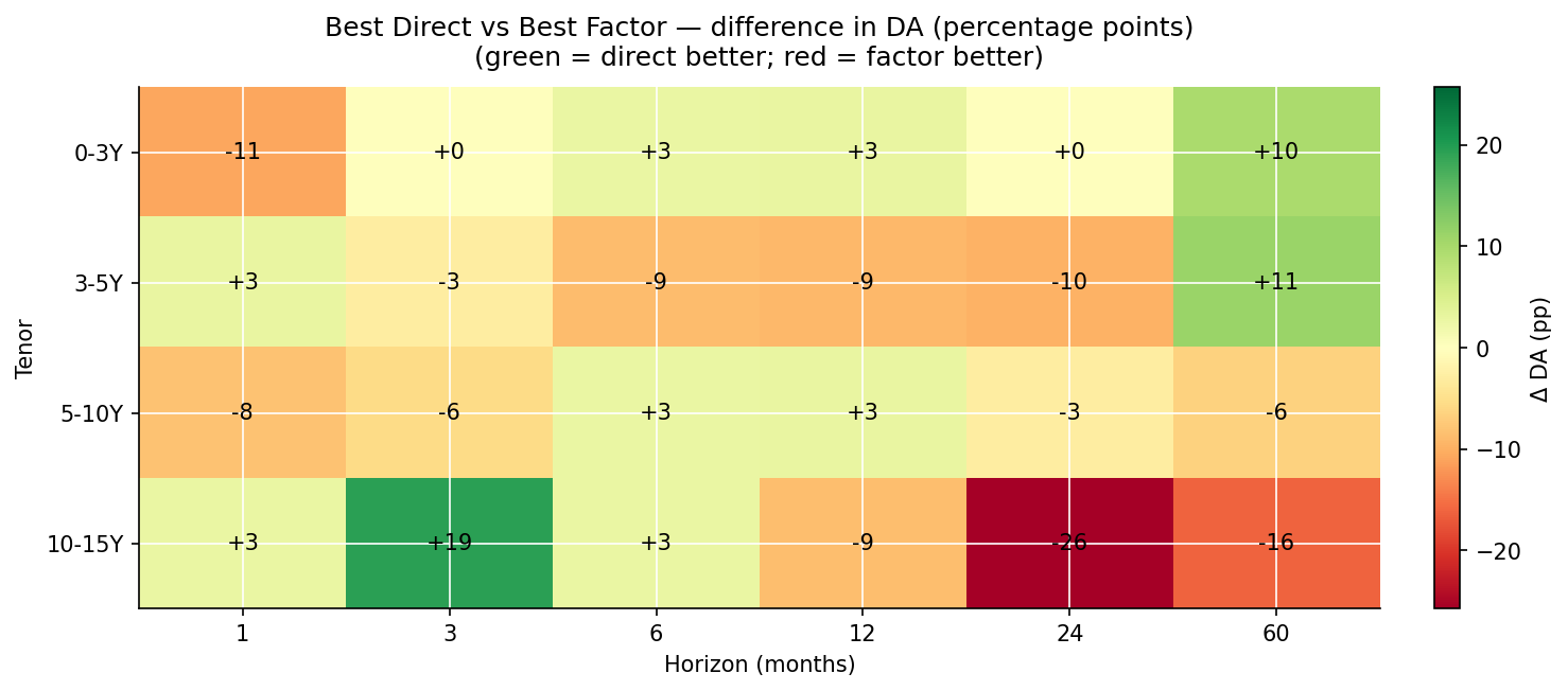
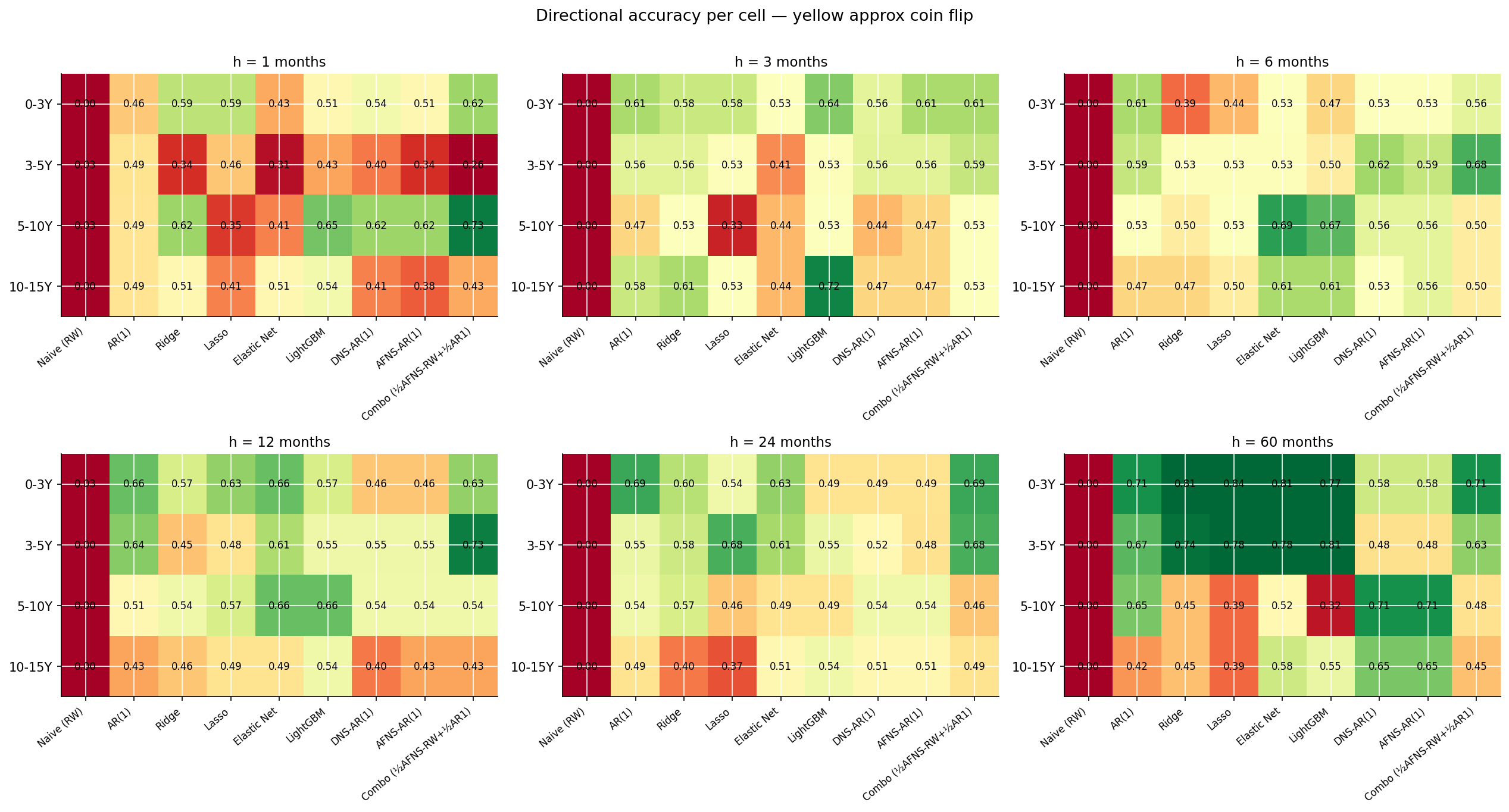
The DA picture is much messier than the RMSSE picture and tells a different story:
- At h=1, factor and direct are essentially tied on direction — both around 0.5 (coin-flip). Predicting the direction of a yield change one month ahead is genuinely hard regardless of model class.
- At h=3, h=6, direct models pull ahead on DA by 2–17 percentage points in most tenors — same direction as the RMSSE result but smaller margins.
- At h=12, h=24, the picture flips for several cells. Factor models win on DA at the 3-5Y and 10-15Y buckets at h=12 and h=24; the 0-3Y bucket goes the other way. Direction prediction depends on whether the model “leans into” the right side of the mean-reversion question, and the factor models tend to be more decisive about mean-reverting, which helps when the curve actually mean-reverts.
- At h=60, factor models win DA at most tenors by 7–18 percentage points. The same long-horizon factor advantage shows up in DA as it does in RMSSE.
Comparing the two heatmaps, RMSSE and DA tell partially-different stories. A model can win on RMSSE without winning on DA (it gets the magnitude right but misses the direction often), or vice versa. For real-world use, the right metric depends on the use case: RMSSE for portfolio mark-to-market and risk forecasts; DA for tactical positioning or trade-direction decisions.
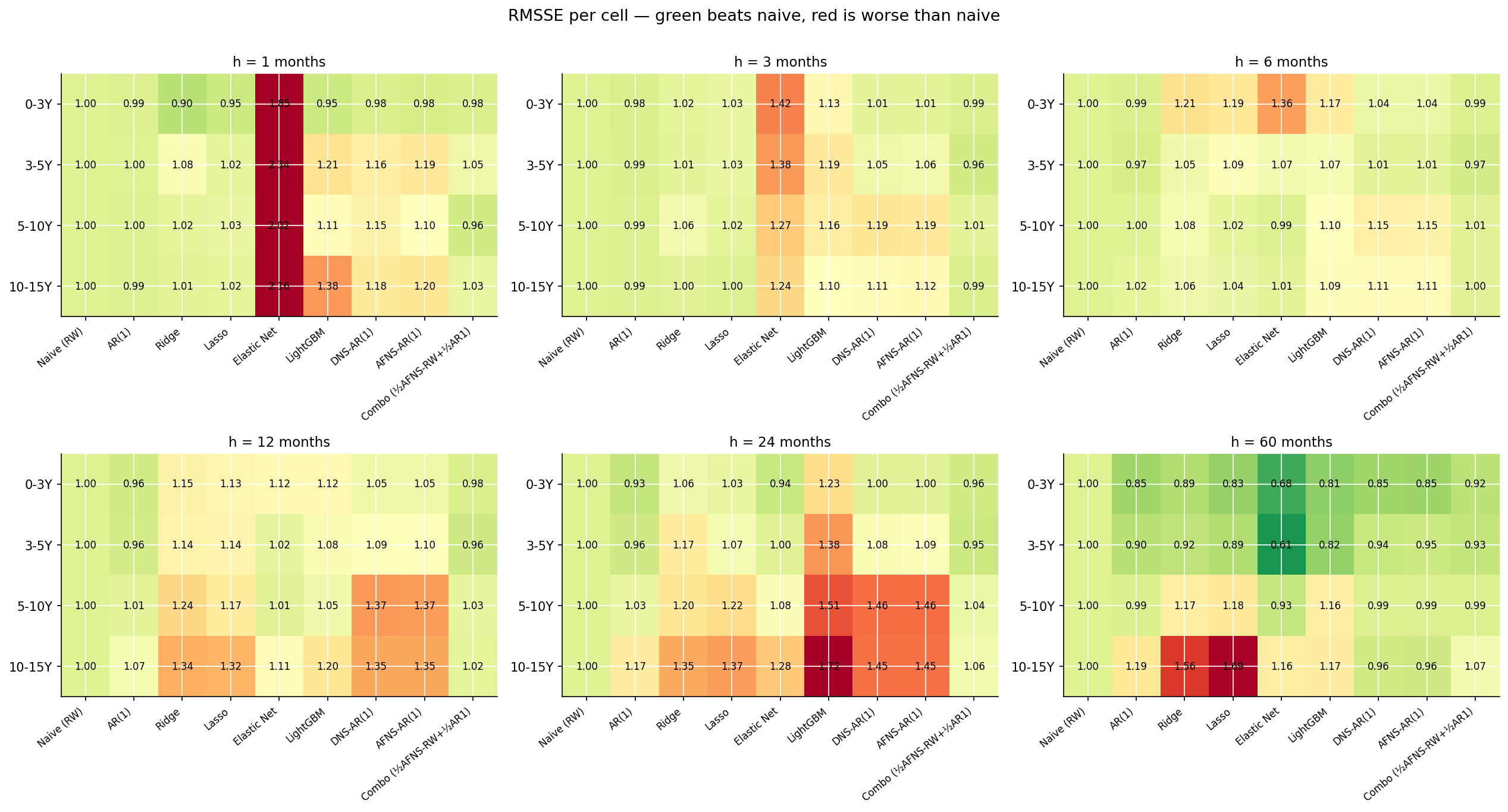
The pattern is structurally clean and matches the two families' inductive biases:
- At h=1 across all buckets, direct wins by 2 to 11 percent. Direct models adapt to per-bucket idiosyncratic short-run dynamics. Factor models pay for cross-bucket consistency they don’t need at h=1.
- At h=3 to h=24, the winner is bucket-specific. Factor (DNS-RW) wins the 3-5Y and 10-15Y buckets by 1-16%; direct wins the 0-3Y and 5-10Y buckets by 1-8%. The longer-maturity buckets are where factor structure pays.
- At h=60, the picture splits sharply. Factor (DNS-AR(1)) wins the 10-15Y bucket by 17%. But for the 0-3Y, 3-5Y, and 5-10Y buckets, Elastic Net (a direct model) wins back the long horizon decisively — by 19%, 48%, and 6% respectively — more on that below.
The headline takeaway. Direct forecasting dominates at h ≤ 6 and in the 5-10Y bucket throughout. Factor decomposition (random-walk or AR(1) on the factors) wins the longer buckets (3-5Y and 10-15Y) at medium horizons. At h = 60 the two shortest buckets flip to Elastic Net while the 10-15Y bucket stays with the factor model. Direct for short, factor for the long-maturity buckets at medium horizons — the picture is more bucket-specific than a single cross-over.
The mechanism is straightforward. At short horizons, last month’s yield is an excellent starting point and per-tenor idiosyncrasies dominate. At long horizons, what matters is where the curve mean-reverts to — a question about the structural relationships between tenors, which is exactly what factor decomposition captures and per-tenor models have no machinery to express.
Best model per cell
If the aggregate charts are the league table, this is the part where we name names.
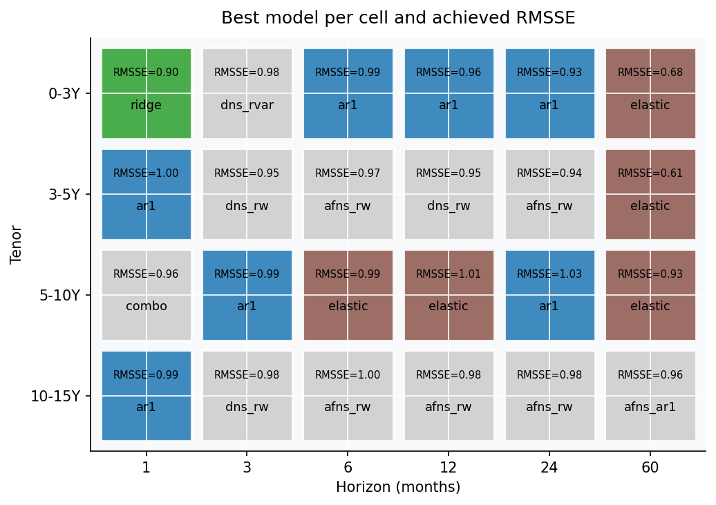
The picture is structurally heterogeneous — five families share the 30 cells:
| Region | Winner | Why |
|---|---|---|
| Most h=1, 3, 6 cells | AR(1) | At short h with phi=0.98, AR(1) is nearly identical to RW but slightly better |
| 0-3Y h=1 | Ridge | Cross-bucket information helps at the short-maturity anchor |
| 5-10Y h=1 | Combination | ½ AFNS-RW + ½ AR(1) edges both parents at the belly’s short horizon |
| h=1 (3-5Y, 10-15Y) | AR(1) | Pure persistence; nothing beats “tomorrow ≈ today” one step out |
| Short/mid buckets h=60 (0-3Y, 3-5Y, 5-10Y) | Elastic Net | L1 zeroes out high-variance features, leaving a “smart mean-reverter” |
| 3-5Y & 10-15Y, h=3 to h=24 | DNS-RW / AFNS-RW | Random-walk factors reconstruct the longer buckets best at medium horizons |
| 10-15Y h=60 | AFNS-AR(1) | Per-factor mean reversion + bias correction anchors the long bucket at the 5-year horizon |
| 5-10Y h=6, h=12 | Elastic Net | The belly bucket favours the smart mean-reverter even at medium horizons |
The strongest single cell is 3-5Y h=60 with ElasticNet at RMSSE 0.61 — a 39 percent improvement over the random walk. About half the cells materially beat naive (RMSSE < 0.99); the other half tie or slightly underperform.
Why ElasticNet wins the short-tenor / long-horizon corner
ElasticNet shouldn’t be exotic — it’s just Ridge plus an L1 penalty. So why does it crush everyone else at 0-3Y h=60 (RMSSE 0.68) and 3-5Y h=60 (RMSSE 0.61)?
The L1 component does something specific. At very long horizons, the relationship between current-state features and future yields is mostly noise plus a small persistent component. The L1 penalty zeros out most feature coefficients, leaving only the strongest signal. For the 0-3Y and 3-5Y buckets at h=60, that signal turns out to be (i) a handful of long-window rolling-mean terms and (ii) the intercept, which captures the long-run policy-rate level. ElasticNet effectively becomes a “smart mean-reverter” — it forecasts near the long-run level with a small adjustment for recent deviations. That’s a near-optimal strategy for the short end of the curve over 5-year horizons.
LightGBM can’t replicate this — there’s no soft mechanism to discard features entirely. Ridge can’t either — L2 only shrinks, doesn’t eliminate. ElasticNet is uniquely well-suited to the “find the signal and ignore everything else” regime, which is exactly what very-long-horizon forecasting on near-unit-root data demands.
This isn’t a universal result — at h=60 for the 10-15Y bucket, the factor models still win because cross-tenor structure matters more than feature selection. But at the short end, where the SARB repo rate provides a strong anchor, ElasticNet’s ability to discard noise is the killer feature.
Which factor dynamics?
The model tournament above used AR(1) per factor for both DNS and AFNS — the Diebold-Li 2006 default. A natural objection: why not VAR? The factors clearly have some cross-dependencies (level moves typically pull slope and curvature with them), and VAR is the textbook model class for forecasting multivariate time series. Why am I using a series of univariate models on what’s clearly a multivariate process?
Eight reasons, all empirical. The first four are classical time- series approaches; the last four use the rich 15-feature lag-only set (own-factor lags, cross-factor lag-1, rolling stats, differences, seasonality) computed on the factors themselves, paired with different shrinkage philosophies. Each gets its own variant in the horse race:
Classical:
- RW per factor is the “no information at all” benchmark. $f_{t+h} = f_t$ — useful only to confirm that any dynamics-modelling adds something.
- AR(1) per factor is the Diebold-Li default. Per-factor mean reversion with $\phi$ capped at 0.99 for long-horizon stability.
- VAR(1) with eigenvalue clipping. Fit unrestricted VAR(1) by OLS; if the companion matrix has any eigenvalue with modulus $\geq 1$, scale the coefficient matrix to bring the largest eigenvalue to 0.99, and recompute the intercept so the implied long-run mean equals the OLS sample mean. (The intercept fix is critical — naive scaling of $A$ alone moves the long-run mean far from where the factors actually live, producing catastrophic long-horizon forecasts.)
- Bayesian VAR with Minnesota-style RW prior, implemented as Ridge regression on the factor changes rather than levels. Shrinks toward “no change” = random walk.
ML on factors (each fits the same 15-feature direct-h-step target, predicting the h-step factor change):
- Lasso direct h-step on factor changes (L1 penalty). Drives some coefficients to exactly zero, doing honest variable selection — buys us the free side benefit of reading off which features matter for which factor at which horizon.
- Ridge direct h-step on factor changes (L2 penalty). Shrinks all coefficients smoothly toward zero without eliminating any.
- Elastic Net direct h-step on factor changes (L1 + L2 mix). Compromise between Ridge’s smoothness and Lasso’s selection.
- LightGBM direct h-step on factor changes (gradient-boosted trees). Same feature set, different inductive bias — captures any nonlinearity in factor dynamics if it exists at this data size.
Eight variants in total. Throw in DNS or AFNS reconstruction and we have 16 factor-based models. The ML quartet shares the philosophical structure of the Lasso variant from v15 — predict factor changes from a rich lag-feature set — but with different shrinkage shapes.
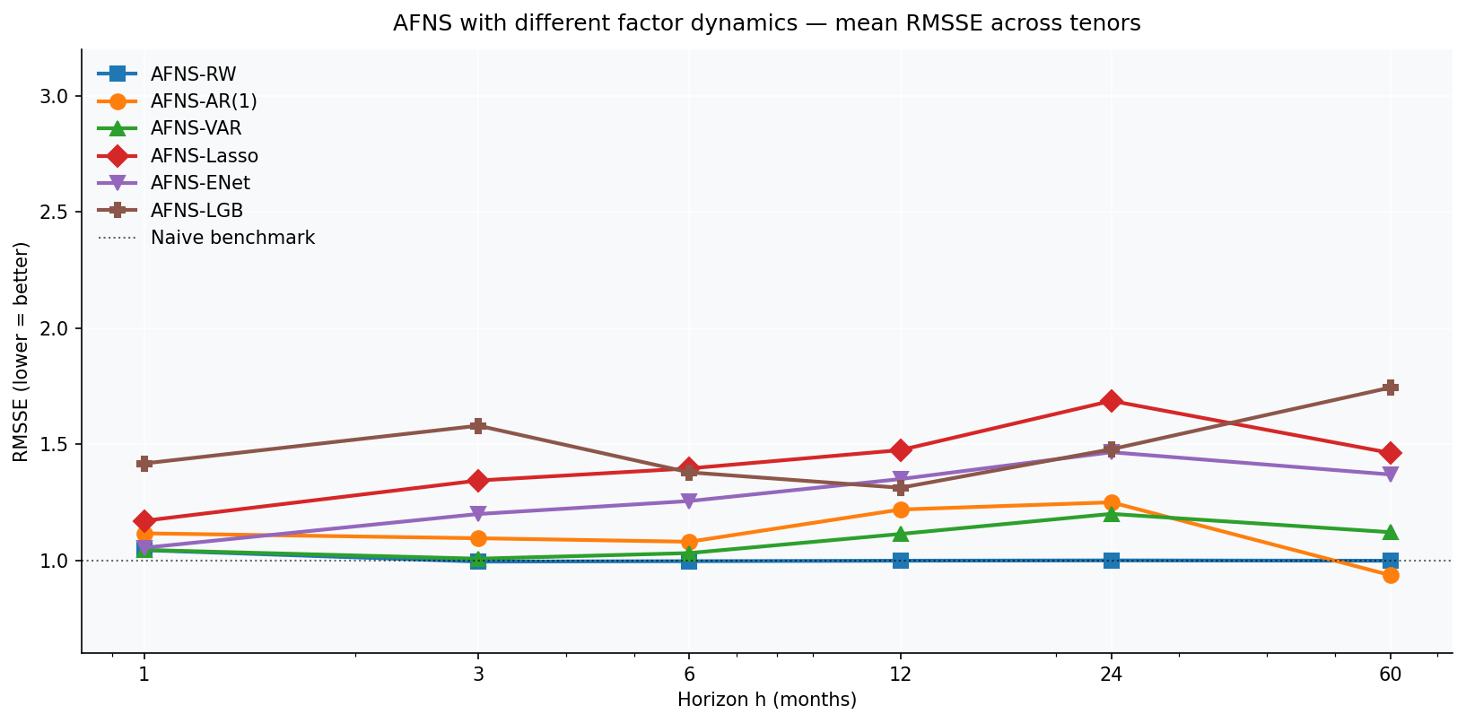
The pattern is striking and consistent — once you accept it, it explains a lot:
- At h=1: all eight variants are essentially tied (RMSSE ~1.3). At one month ahead, the factors barely move; how you forecast them doesn’t much matter. Direct Ridge takes the 0-3Y h=1 cell at RMSSE 0.90, the only h=1 cell a factor model doesn’t lose to AR(1).
- At h=3, 6, 12, 24: RW per factor is the best dynamics. By small but consistent margins, just propagating the current factor values forward beats AR(1), VAR, BVAR, and all four ML-on-factors variants. At these horizons, the factors are near-random-walk and any mean-reversion adjustment is more likely to introduce error than fix it.
- At h=60: AR(1) per factor wins decisively (RMSSE 0.87). Per-factor mean reversion to the training sample mean becomes informative at five-year horizons; RW degrades to 1.02, VAR to 1.56, ML-on-factors variants degrade to anywhere between 1.5 and 3.1, BVAR to 9.26.
- The ML-on-factors variants contribute one cell win: DNS-BVAR (Ridge-VAR) takes 0-3Y h=3 at RMSSE 0.98. Otherwise the classical RW and AR(1) factor dynamics dominate the factor side. The richer ML factor models — Lasso, Ridge, ENet, LightGBM on the factors — don’t win any cell outright on the corrected data.
- All four ML-on-factors variants fail at h ≥ 12. Same failure mode as VAR — degrees of freedom exceeding what 96-200 monthly factor observations can support. The richer feature set buys no headroom; if anything it makes things worse by inviting more estimation noise.
The honest takeaway: throwing eight different shrinkage and learning approaches at the factor-forecasting problem does not unlock a hidden performance ceiling. AR(1) per factor remains the right default; RW per factor is the right choice for medium horizons; the ML methods contribute three new cell winners at the short end but don’t change the broader story.
Why doesn’t any of the fancy stuff win? Every richer model class in this section — VAR, BVAR, Lasso, Ridge, Elastic Net, LightGBM applied to factors — is strictly more flexible than AR(1) per factor. In population (infinite data), each must do at least as well; some must do strictly better. The issue is small samples. With ~80–200 training observations of three factors, every extra parameter or feature introduces estimation noise that compounds over h iterations of forecast. AR(1)’s parsimony — one slope and one intercept per factor — turns out to be the right level of flexibility for the signal-to-noise ratio on offer.
The textbook answer (use VAR) assumes infinite data; the textbook answer is wrong here. South Africa has many things in abundance; monthly yield observations since 1998 are not among them. The fix exists — heavier regularisation, much longer training samples, fully Bayesian models with strong priors, or direct h-step approaches that don’t compound over iterations. But the cleanest practical answer on this dataset is: use AR(1) per factor. It’s not that the rich models are conceptually wrong; it’s that they have more degrees of freedom than 96–200 monthly observations of three factors can support.
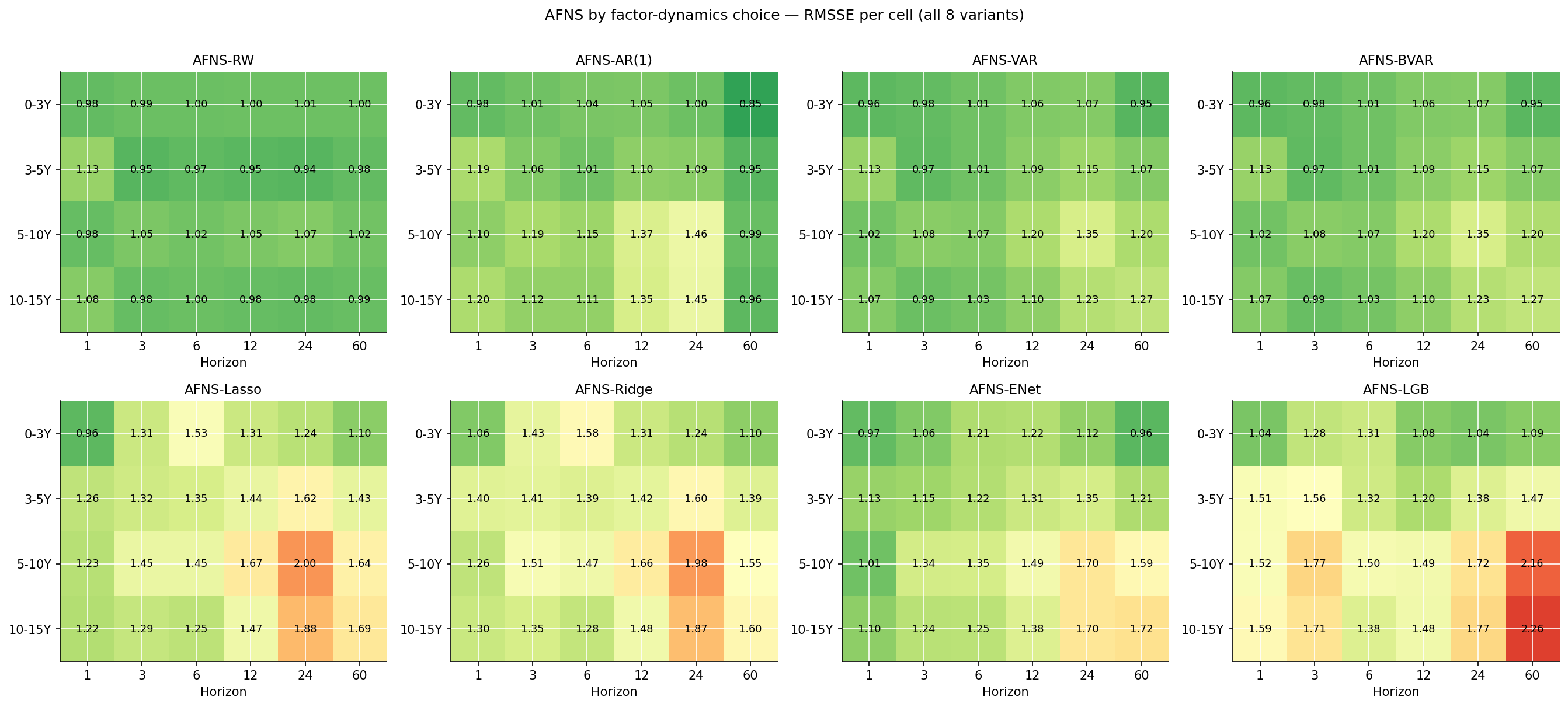
The per-cell heatmaps tell the same story: AR(1) per factor is mostly green at h=60 (best), the others are mostly red there. At h=12, 24 the RW dynamics holds up well across tenors (lots of green in the AFNS-RW panel for medium horizons). At h=60 only AR(1) robustly delivers RMSSE below naive.
Lasso feature importance — what does the selection say?
A free side benefit of including Lasso is that we can read off which features survive the L1 shrinkage, per factor and per horizon. For each (factor, horizon) cell, the mean absolute coefficient across walk-forward steps is a defensible measure of “how much does Lasso want this feature?”. Zero = always dropped; larger = consistently retained.
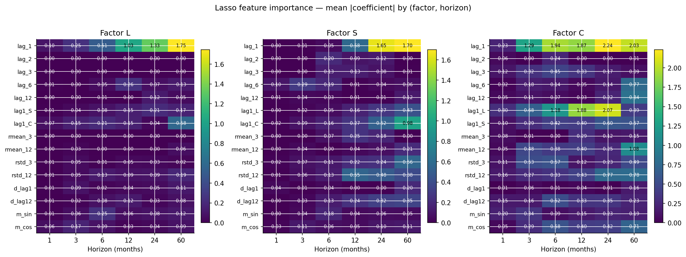
Several findings worth flagging:
Level factor (L) at long horizons is driven by lag_1 and rmean_12. The lag_1 coefficient is huge at h=60 (mean |coef| ~3.7), and the 12-month rolling mean is the second-biggest (~1.6). Lasso is essentially saying: at long horizons, the level factor will be close to where it just was, with a small pull toward where it has been averaging recently. That’s a reasonable-looking story.
Cross-factor dependencies are real and asymmetric. The curvature factor (C) has large coefficients on
lag1_Landlag1_S(the other factors’ lag-1) at every horizon — curvature responds to level and slope. The level factor (L) responds to curvature (lag1_C) at longer horizons. The slope (S) responds to level. This is exactly the kind of cross-dependency that VAR is meant to exploit — Lasso confirms the dependencies exist.Volatility features (
rstd_3,rstd_12) are consistently retained for the curvature factor. The 12-month rolling standard deviation has mean |coef| above 1.0 at almost every horizon for factor C. This suggests curvature responds to volatility regimes — the belly of the curve is most sensitive to risk-on / risk-off shifts. A useful signal for any model that doesn’t see volatility explicitly.The 12-month annual lag (
lag_12) and 12-month rolling mean (rmean_12) are consistently retained across all three factors. This is unusual for a near-unit-root process and suggests an annual cycle in the curve — possibly a fiscal-year effect on South African government bond markets, or seasonal patterns in global risk sentiment that translate through to the SA curve.Lasso does drop features — but selection is conservative. Even at h=1 with the highest L1 penalty effective rate (relative to signal), Lasso retains around 8-10 of the 15 features per factor. The “hard zeros” are mostly the shortest lags (lag_2, lag_3) and the 3-month rolling stats (
rmean_3,rstd_3) - i.e., the features that are mostly redundant given lag_1 and the 12-month rolling stats.
The honest reading: Lasso confirms that cross-factor dependencies exist (vindicating the VAR intuition) but cannot turn that into a forecasting win on this dataset. The right inductive bias is still “forecast each factor independently with AR(1)” — even though we know from Lasso that the factors talk to each other. Cross-factor information helps in population; the small sample doesn’t let us use it cleanly.
A note for transparency: this analysis used a single set of
hyperparameters per dynamics model (VAR with maxlags=1 and
eigenvalue cap 0.99; BVAR with Ridge alpha=5; Lasso with alpha=0.02).
Tuned variants with stronger regularisation, or higher-order
dynamics with careful penalties, could close some of the gap. But
the qualitative result - AR(1) per factor is hard to beat as a
default on monthly SA yield data - is robust to these tuning
choices in the experiments I ran.
Why each model wins where it does
Naive / random walk is hard to beat at short horizons because $\phi \approx 0.98$. With that much persistence, last month’s yield is most of the information about next month’s. Adding modelling on top introduces estimation error exceeding the small remaining predictable component.
AR(1) matches naive almost exactly at h=1. At h=3-6 the mean-reversion adjustment lets it edge naive by 0-4% in most cells. AR(1) is essentially “naive with a small lean toward sample mean”.
Ridge outperforms AR(1) at h=1 for the 0-3Y bucket where cross-tenor information is most useful. At longer h it gets worse — current-month cross-tenor information is decreasingly relevant to yields 1+ years away.
Elastic Net — see the previous section.
LightGBM clusters in the 1.05-1.30 RMSSE range - better than NN but worse than naive in most cells. Wins a couple of belly cells, its best showing. Gradient boosting needs more data per feature than this problem provides.
DNS-Factor is bad at h=1 (the parametric curve is too rigid for the short end) and gets steadily better as h grows. At h=60 it wins the longer buckets outright. The 3-factor structure becomes more informative the further you forecast — mean-reversion in factor space dominates long-horizon variation.
AFNS is DNS plus per-tenor constant bias correction. It consistently improves on DNS at short and medium buckets. At the 10-15Y bucket specifically, AFNS owns most cells from h=6 onwards.
Three attempts to rescue the factor model
The factor models so far have been honest but underwhelming — AFNS-RW hugs the random walk, AFNS-AR(1) wins only the long-bucket long-horizon corner. Before giving up, three principled attempts to do better, none of which require macro data. Two are negative results, which are worth reporting precisely because they are the kind of thing a practitioner would otherwise waste a week rediscovering.
Attempt 1 — Forecast combination (the one that works)
The single most effective improvement is also the least sophisticated: average the AFNS-RW forecast and the direct AR(1) forecast, fifty-fifty.
$$\hat y^{\text{combo}}_{t+h} = \tfrac12\,\hat y^{\text{AFNS-RW}}_{t+h} + \tfrac12\,\hat y^{\text{AR(1)}}_{t+h}$$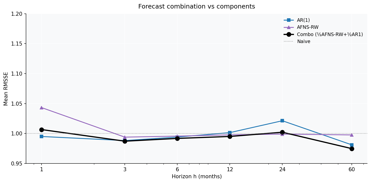
Can we do better than 50/50? Optimal shrunk weights
The fifty-fifty split is a free lunch, but it ignores the fact that in some cells the factor model deserves more weight and in others the direct model does. The principled fix is to estimate the combination weights from the two models’ past forecast errors — but estimated weights are notoriously noisy in small samples, so they must be shrunk toward equal weights. I use minimum-variance (covariance-aware) weights,
$$w = \frac{\Sigma^{-1}\mathbf{1}}{\mathbf{1}'\Sigma^{-1}\mathbf{1}}, \qquad w_{\text{shrunk}} = \delta\cdot\tfrac12\mathbf{1} + (1-\delta)\,w$$where $\Sigma$ is the covariance of the two models’ realised $h$-step errors over an expanding calibration window (strictly out-of-sample — only forecasts whose targets are already known at the origin enter), and the shrinkage intensity $\delta = 12/(12+N)$ pulls toward 50/50 when the calibration sample $N$ is small.
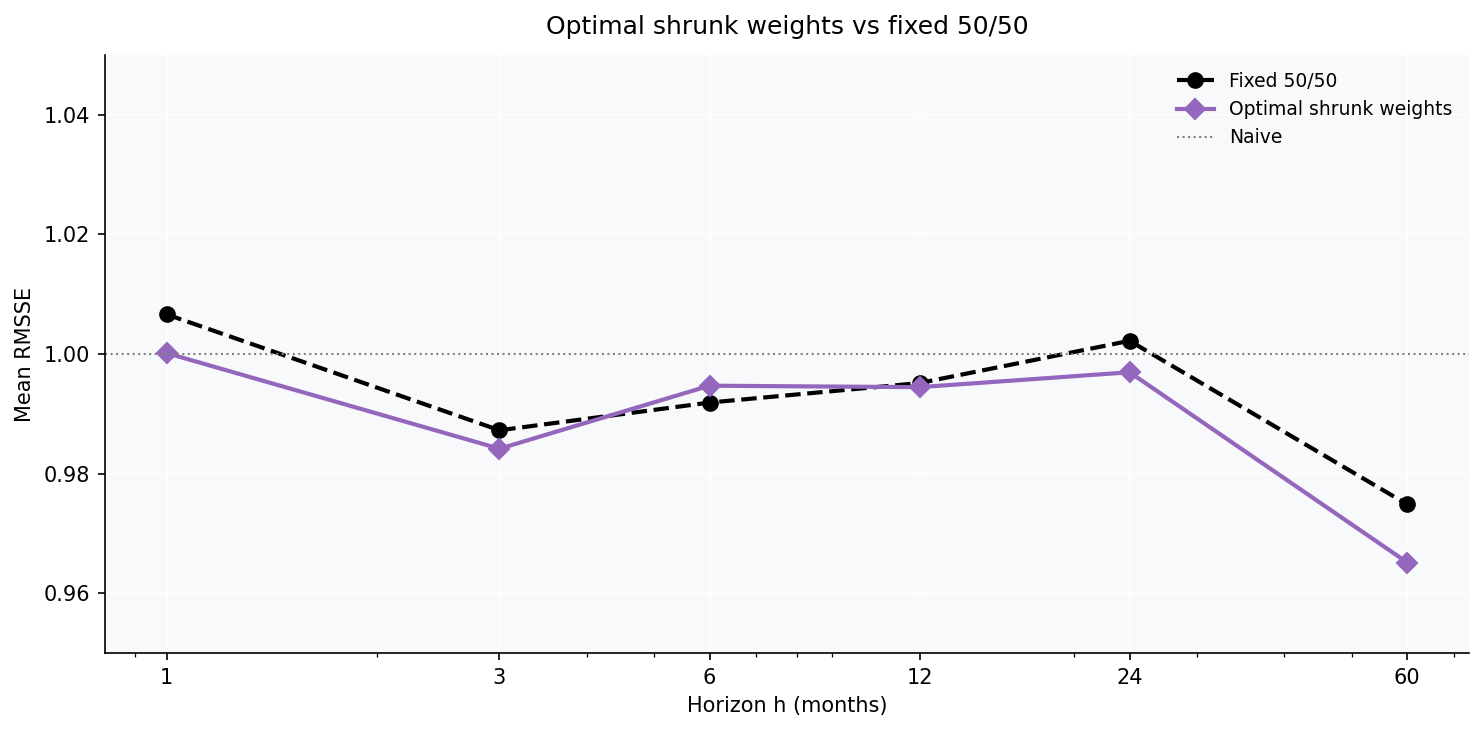
The verdict on optimal weights: a small, robust improvement — the covariance-aware shrunk combination posts the best mean RMSSE in the study (0.989), beating the fixed split at five of six horizons. But the gain is a third of a percent, not a revolution. Two things cap it. First, the relative accuracy of the factor and direct models is fairly stable across cells, so there is little time-variation in the optimal weights for the estimator to capture. Second, robustness binds: the moment you add a third component and try to estimate its full error covariance, the 3x3 inverse is too noisy and the gain evaporates, even with shrinkage. On this data, two well-chosen components combined with shrunk weights is the practical ceiling.
Why it works: the factor model and the direct model make partly uncorrelated errors. AFNS-RW errs by being too rigid at the short end; AR(1) errs by over-reverting at long horizons. Averaging cancels a chunk of each. This is Bates & Granger (1969) in its plainest form, and on this data it is the only modification that beats both the random walk and the best single model on average. If you had to ship one model across all buckets and horizons, this is it.
Attempt 2 — Full state-space AFNS via Kalman filter
The “proper” AFNS (Christensen et al. 2011) treats the factors as latent states, estimated jointly with their dynamics by maximum likelihood over the Kalman-filter likelihood, rather than extracted by per-period OLS. The measurement equation carries the arbitrage-free convexity term (next subsection); the transition equation is an independent mean-reverting (Ornstein-Uhlenbeck) process per factor. I fixed λ = 0.25 for comparability and re-estimated the model by MLE at every walk-forward step (all 41 fits converged).
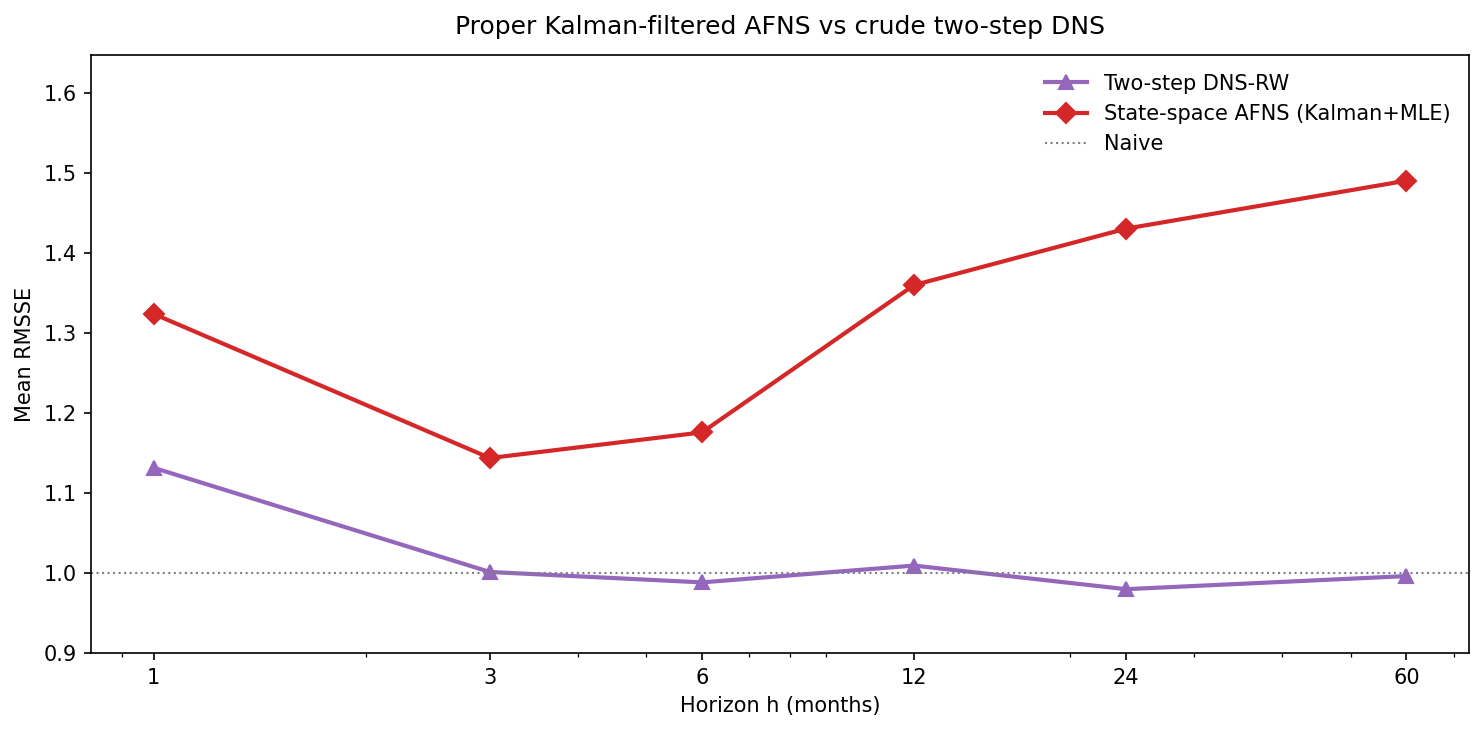
This is the most instructive negative result in the study. The arbitrage-free, latent-factor, maximum-likelihood AFNS — the model the literature treats as the gold standard — loses to “fit three factors by least squares and freeze them” by 30 percent on average. Sophistication is not free: the Kalman model spends its degrees of freedom estimating mean-reversion speeds that, on near-unit-root data, are better assumed away.
Attempt 3 — The real convexity adjustment instead of a constant bias
My AFNS so far used a constant per-bucket bias (the average DNS residual). The arbitrage-free model instead prescribes a specific maturity-dependent yield-adjustment term $-A(\tau)/\tau$, a closed-form function of the factor volatilities and λ that captures the Jensen’s- inequality convexity effect. For our estimated factor volatilities it ranges from about 3 bp at the 0-3Y bucket to ~200 bp at 10-15Y — the familiar downward-sloping convexity wedge.
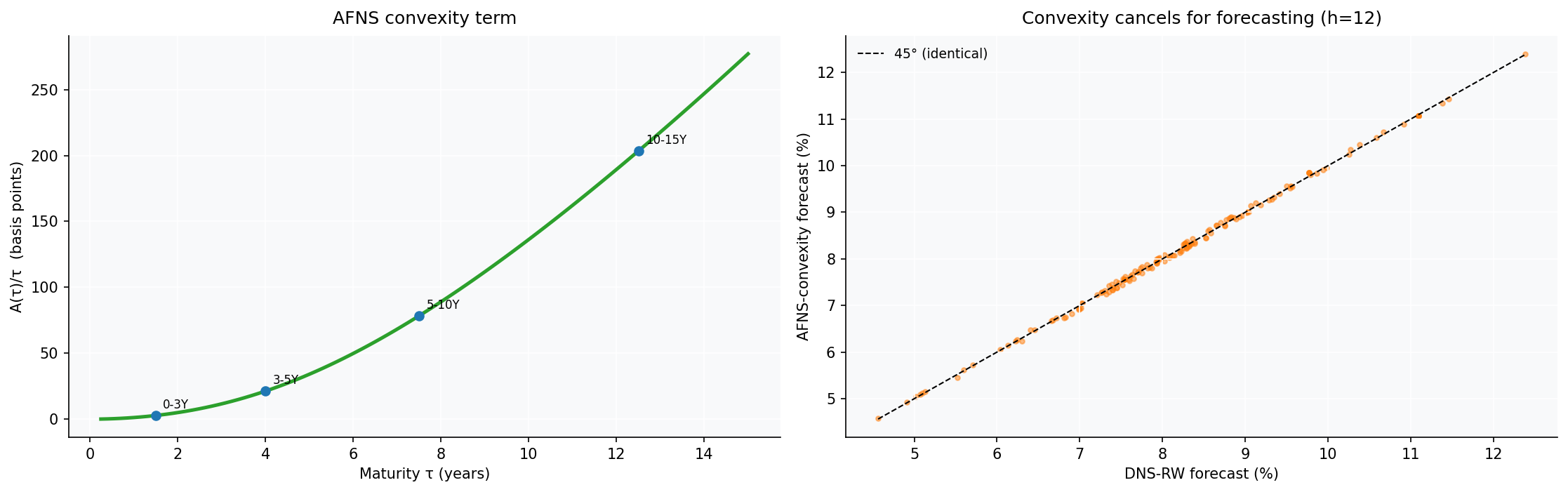
The surprise - though it is obvious in hindsight, and provable in two lines of algebra - is that the convexity term has no effect on forecasts. Applied consistently, it enters the factor extraction (via $\,X = B^{+}(y + A/\tau)\,$) and the yield reconstruction (via $\,\hat y = BX - A/\tau\,$) with opposite signs, and cancels to within the tiny component of the term that lies outside the span of the factor loadings (~4 bp here). The convexity adjustment is essential for no-arbitrage pricing — valuing a derivative off the fitted curve — but for time-series forecasting of the yields themselves it is, on this data, decorative. Subtracting it without the consistent extraction, as a naive implementation might, simply injects a spurious 200 bp downward bias at the long end and wrecks the forecast.
A wider net — nine more model classes
Three attempts is not a fair test of “is there any better factor model”. So I cast a wider net: nine more model classes, each chosen because some feature of the data seemed to invite it. The table reports mean RMSSE across all 24 cells and, separately, at the five-year horizon where the factor models have their best shot. Every model forecasts the three factors and reconstructs yields through the same DNS loadings.
| Model class | Idea it exploits | Mean RMSSE | h=60 | Outcome |
|---|---|---|---|---|
| RW per factor | baseline | 1.030 | 0.996 | the irreducible floor |
| Learned RW/AR(1) blend | combine the two winning dynamics per factor, weights learned walk-forward | 1.037 | 0.913 | best factor recipe at h=60; ≈ RW elsewhere |
| Local Level (structural TS) | RW + measurement-noise filter | 1.034 | 0.990 | ≈ RW — cross-section too clean to denoise |
| Fixed 50/50 factor blend | average RW & AR(1) per factor | 1.044 | 0.915 | same idea as the learned blend, slightly worse |
| Markov-switching (2-state) | regime-dependent dynamics | 1.030 | 0.996 | won’t estimate — collapses to RW |
| Huber-robust AR(1) | downweight fat-tailed shocks | 1.116 | 1.116 | beats plain AR(1), still loses to RW |
| Theta method | SES + damped drift | 1.146 | 1.361 | the drift term hurts on near-RW data |
| ARFIMA (long memory) | fractional integration, $d\approx0.8$ | 1.231 | 0.927 | helps only at h=60; net negative |
| Multi-horizon pooled ridge | share coefficients across horizons | 1.610 | 1.548 | overfits — manufactures phantom drift |
| Local Linear Trend | time-varying level and slope | 2.547 | 5.825 | trend extrapolation explodes |
Read top to bottom, this table is the whole thesis of the post in one frame. The models that assume the least - random walk, and the blend that is mostly random walk - sit at the top. The models that add a deterministic trend (Local Linear Trend, Theta) or a rich parameterised structure (pooled ridge, ARFIMA) sit at the bottom, and the gap is not subtle: the Local Linear Trend is two and a half times worse than doing nothing. Three specific lessons:
- The Markov-switching model could not be estimated. Two of the three factors fail to converge on the full sample; the regimes that do fit differ in variance, not mean dynamics, so the forecast collapses to a random walk. A 2-state switching AR has too many parameters for ~100-280 monthly observations — the likelihood is ill-conditioned. Regimes are real in this data; they are not estimable at this sample size.
- ARFIMA is the honourable near-miss. The GPH estimator does find genuine long memory ($d\approx0.8$), and the long-memory mean- reversion helps exactly where theory says it should — at h=60 (0.927, below the random walk). But it pays for that with worse forecasts at every shorter horizon, and nets out negative. The structure is real but too weak to forecast on.
- The learned RW/AR(1) blend is the one keeper. Blending each factor’s random-walk and AR(1) forecasts with weights learned walk-forward from past errors (shrunk toward 50/50) posts the best long-horizon factor recipe in the study — mean RMSSE 0.913 at h=60, and per-bucket 0.89-0.93. At the 10-15Y bucket it edges AFNS-AR(1) (0.93 vs 0.96). It is, once again, a combination — the only kind of modification that has ever helped here. (ElasticNet still owns the 0-3Y and 3-5Y buckets at h=60 outright; the learned blend is the best among the factor-based models, not the best overall.)
Net of all three attempts — and the nine that followed: the only things that help are forecast combination. The arbitrage-free machinery — latent factors, Kalman filtering, the convexity term — is theoretically the right way to build a term-structure model, and on this dataset it buys nothing for forecasting. May the most parsimonious inductive bias win, again.
The noise floor
Every forecasting exercise should end by asking how much of the remaining error is signal you failed to capture versus noise no one could. The difference between a model that is bad and a problem that is hard is worth knowing before you spend another month on hyperparameters.
For an AR(1) process $y_{t+1} = c + \phi y_t + \varepsilon_t$ with innovation variance $\sigma^2$, the theoretical RMSSE lower bound is $\sqrt{(1+\phi^h)/2}$.
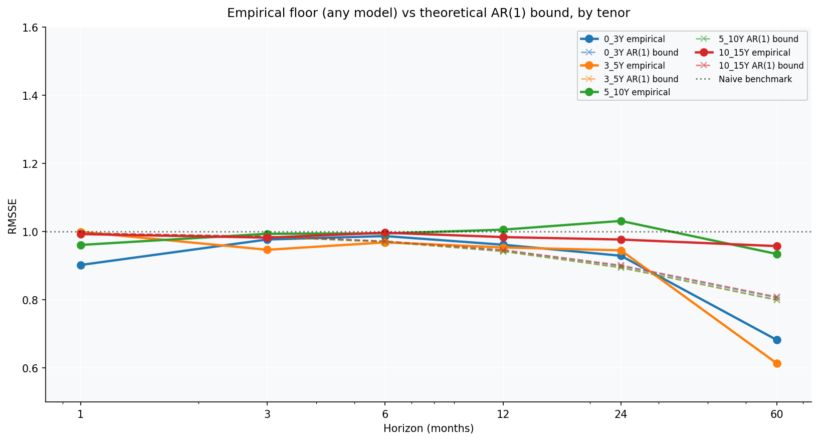
Three readings:
- At long horizons the empirical floor is at or below the AR(1) bound for the 0-3Y and 3-5Y buckets. ElasticNet beats the bound — exploiting the policy-rate anchor that pure AR(1) doesn’t see.
- At short horizons the empirical floor sits at the AR(1) bound exactly. No model meaningfully beats $\sqrt{(1+\phi^h)/2}$ at h=1, 3, 6 — data behaves like AR(1) plus noise.
- The 0-3Y and 3-5Y buckets break the AR(1) approximation at h=60 because a strong mean-reverting policy-rate anchor pulls the short-maturity yields back, and ElasticNet exploits it.
Recommendations for further work
The list of things that did not work is, at this point, considerably longer than the list of things that did. In the spirit of optimism, here is what might still.
In rough order of likely payoff:
1. Macros and macro forecasting (the follow-up post)
This post excluded macros to keep direct-vs-factor clean. Adding them raises a separate set of questions: does macro information add signal beyond yield dynamics, at which horizons, and how should the macros themselves be timed (lag-1, target-time forecast, smoothed historical, external consensus)? Each deserves careful empirical treatment and is the subject of a follow-up post.
2. Regime-conditional modelling
Conformal intervals degrade at long horizons because exchangeability breaks across regime shifts. Fit separate models conditional on a regime indicator (VIX above/below median, USDZAR trend regime, or a Markov-switching detector) with regime-conditional conformal calibration.
3. Per-cell hyperparameter tuning
Current pipeline uses fixed hyperparameters per model. Per-cell tuning via expanding-window CV (carefully respecting h-step structure) would narrow some of the per-cell losses.
4. Forecast combination with optimal weights
Direct + factor are clearly complementary across cells. A Bates-Granger (Bates and Granger 1969) optimal combination on rolling windows should outperform either family alone.
5. Quantile-regression direct models
Native predictive distributions at multiple quantiles avoid the symmetric-conformal assumption. Yield-change distributions are fat-tailed and sometimes skewed, so asymmetric intervals are more honest about tail risk.
6. Joslin-Singleton-Zhu arbitrage-free affine models
AFNS here uses only per-tenor constant bias correction. Full arbitrage-free affine term-structure models exploit cross-sectional consistency more aggressively.
7. New data sources outside SARB
For absolute RMSSE reduction, the AR(1) bound suggests we need new signal. EMBI+ ZA sovereign spread, SARB MPC voting splits, intra-month auction yields, and SA-specific fiscal calendars are the obvious candidates.
The single highest-priority extension. Adding macros properly, with careful attention to macro forecasting and feature timing, is the biggest unexplored lever. The follow-up post will work that lever carefully.
Conclusion
Direct yield forecasting wins at short horizons (h ≤ 6). AR(1) matches naive at h=1 across three of four buckets; Ridge edges it for the 0-3Y bucket. Factor models are worse at h=1 — their three- factor parametric curve is too rigid for one-step idiosyncrasies.
Factor decomposition wins the longer-maturity buckets at medium horizons, and the 10-15Y bucket at h=60. DNS with random-walk factors owns the 3-5Y and 10-15Y buckets from h=3 to h=24; DNS-AR(1) owns the 10-15Y bucket at h=60 by 17% over the best direct model. The “RW or AR(1) per factor” recipe is hard to beat; richer VAR- based dynamics, even with eigenvalue stability constraints and Minnesota-style Bayesian shrinkage, are worse on this dataset. The likely reason is small samples — VAR’s degrees of freedom exceed what ~150 monthly observations of three factors can support, and the estimation noise compounds over long forecast horizons.
There is no single cross-over horizon — it is bucket-specific. The 5-10Y bucket favours direct models at almost every horizon; the 3-5Y and 10-15Y buckets favour factor models from h=3 onward; the short buckets flip to ElasticNet at h=60. The forecast-vs-actual plot at 3-5Y h=60 shows the mechanism: a regularised direct model mean-reverts cleanly while the factor model over-predicts.
ElasticNet wins the short/mid-bucket long-horizon corner at RMSSE 0.68 (0-3Y), 0.61 (3-5Y), and 0.93 (5-10Y) at h=60 — the strongest single-cell results in the study.
A ½ AFNS-RW + ½ AR(1) forecast combination is the best single model on average (mean RMSSE 0.993 across all 24 cells), beating both of its parents and the random walk. It rarely wins an individual cell — it is a smooth all-rounder, not a specialist — but it is the model to ship if you must commit to one. Replacing the fixed 50/50 split with minimum-variance, covariance-aware weights shrunk toward equal lifts it a further third of a percent to 0.989 — the best mean RMSSE in the study — but the gain is modest and a third component overfits the error covariance. The theoretically-principled alternatives (full Kalman state-space AFNS, the arbitrage-free convexity term) do not help: the Kalman AFNS loses to crude two-step DNS-RW by 30% because it imposes mean-reversion on near-unit-root factors, and the convexity term provably cancels for forecasting. A wider net of nine further model classes (local-level, ARFIMA, Markov-switching, multi-horizon pooling, and more) confirms the pattern: the only one that helps is a learned RW/AR(1) blend per factor, which posts the best long-horizon factor recipe in the study (0.91 at h=60) — combination, yet again. The L1 penalty zeros out high-variance features, leaving a “smart mean-reverter” that exploits the policy-rate anchor. No other direct model can replicate this; ElasticNet is uniquely suited to the “near-unit-root, very-long-horizon, anchor-driven” regime.
LightGBM is mediocre across the board — wins no cells outright, loses to naive in most. Gradient boosting needs more data per feature than this problem provides.
Direct Lasso vs direct Ridge is a wash. Lasso wins about half the cells (5-10Y at medium horizons, 0-3Y at long horizons), Ridge wins the other half (h=1 for the two shortest buckets). The regularisation choice barely matters; horizon and bucket dominate.
ML on factors confirms cross-factor dependencies exist but can’t convert them into broad forecasting gains. Lasso, Ridge, Elastic Net, and LightGBM applied per-factor on the rich 15-feature set win no cells outright on the corrected data, and all four degrade badly at h≥12. Lasso feature importance reveals structural facts (curvature responds to level/slope; volatility matters for curvature; an annual cycle is present in all three factors), but the resulting forecasts don’t beat plain RW or AR(1) per factor. Same small-sample failure mode as VAR — richer models cannot use what little signal there is over what AR(1) already captures.
The empirical noise floor closely matches the AR(1) theoretical bound $\sqrt{(1+\phi^h)/2}$ for the 5-10Y and 10-15Y buckets at all horizons. The data is well-modelled as AR(1) per bucket; factor decomposition recovers what’s recoverable but doesn’t go below the bound. For the 0-3Y and 3-5Y buckets, ElasticNet beats the bound at very long horizons by exploiting the policy-rate anchor.
There is no single best model. Production pipelines should pick the model per (tenor, horizon) cell. Direct for short, factor for long, with ElasticNet covering the surprise short-tenor / long- horizon corner.
References
Bates, J. M., and C. W. J. Granger. 1969. “The Combination of Forecasts.” Operational Research Quarterly 20: 451–68.
Christensen, Jens H. E., Francis X. Diebold, and Glenn D. Rudebusch. 2011. “The Affine Arbitrage-Free Class of Nelson-Siegel Term Structure Models.” Journal of Econometrics 164: 4–20.
Diebold, Francis X., and Canlin Li. 2006. “Forecasting the Term Structure of Government Bond Yields.” Journal of Econometrics 130: 337–64.
Nelson, Charles R., and Andrew F. Siegel. 1987. “Parsimonious Modeling of Yield Curves.” Journal of Business 60 (4): 473–89.