Shorter Than You Booked
Why bother
A South African bank funds itself largely with current accounts and savings deposits. Those balances have no maturity - a depositor can walk into a branch tomorrow and take the lot - but in aggregate they barely move, and the rate paid on them lags the repo rate rather than tracking it. The bank is sitting on a very large pool of money that is contractually overnight and behaviourally long, and it has to decide what to do about that.
Take a bank with R100bn of non-maturing deposits. I will carry that example the whole way through, because every ratio in this post turns into a rand figure once you have it.
Post 2 measured how much of a repo move this bank passes on to depositors. The answer is β = 0.489. So when the SARB hikes 100bp: assets reprice almost immediately and earn an extra R1,000m, deposits cost an extra R489m, and net interest income rises R511m.
That R511m is the entire problem in one number. It is a windfall when rates rise and an identical hole when they fall, and South African rates do not move politely - over our sample the repo ranged from 3.50% to 12.00%. A bank that does nothing is running an unhedged R511m-per-100bp position on the SARB’s mood, and the year-on-year swing in its net interest income has a standard deviation of about R828m.
Ask a desk how the programme is designed and you will hear a version of this: one hundred and twentieth of the book matures each month, reinvested at the ten-year swap rate, so the yield is a ten-year moving average. RBS described its programme in exactly those terms. Barclays’ teach-in describes the same mechanics. It is sensible, legible, and very widely copied.
It is also, quite literally, a boxcar filter - the crudest low-pass filter in signal processing, the one every textbook uses as the example of what not to build. So this post takes the observation seriously: estimate what South African rates actually do, work out what the boxcar does to it, and solve for the filter that would do it better.
What I found
Three things came out sideways, and they are the post.
There is no rate cycle to design against. The South African short-rate spectrum has no peak. It is a shelf that rises with period and flattens past ten years, because the SARB’s big moves are responses to shocks - the financial crisis, the pandemic, the inflation surge - and shocks do not arrive on a schedule. There is no bump for a cleverer filter to notch out.
The optimiser handed back the design the industry already uses. Solve for the best possible weighting of past rates, and the answer is a uniform ladder at the longest tenor available. The gain from reshaping is 0.00 basis points. That is not a failure of the optimisation; it is a small theorem, and I can now say why the caterpillar is right rather than merely that it is common.
A growing deposit book quietly shortens the hedge by a third. Every published treatment of a caterpillar I are aware of - ours included, until I checked - assumes a constant deposit base. Real programmes maintain notional as a percentage of a book that grows, so old tranches shrink as a share of today’s balance. At the growth rate I measured, a twenty-year programme behaves like a seven-and-a-half-year one.
What it is worth
A great many structural hedge programmes sit somewhere near 40% of the non-maturing book at around five years. Starting there, on our R100bn example:
| Decision | earnings volatility | income per year |
|---|---|---|
| size it at 49% instead of 40% | −R8m | +R80m |
| run it at fifteen years, not five | −R160m | +R1104m |
| build it from bonds rather than swaps | R0m | +R778m |
| reshape the ladder | R0m | R0m |
| all together | −R168m | +R1962m |
That is roughly 39% less earnings volatility and about R2.0bn a year of additional income, on a deposit book of R100bn. Scale it to a South African major and the tenor decision alone is a multi-billion-rand line item that no committee is currently voting on, because it is buried in a programme description rather than presented as a choice.
The tenor decision is the largest single lever, which surprised us - it beats the instrument decision by a comfortable margin. Lengthening from five years to fifteen roughly triples the term premium collected and smooths over three times as many past rates, so it is one of the rare changes that improves both axes at once.
What is different about this
Most of what follows is an argument that existing practice is right. That is worth saying plainly, because the two things that are genuinely new are narrow.
The framing is borrowed wholesale from signal processing, and that is the point: a rolling ladder is a finite impulse response filter, so the question “what is the best ladder?” becomes “what is the best filter?”, which has a literature and a set of tools. What that buys is not a better ladder - it is a proof that the uniform one is optimal within the class a spot programme can build, where the industry has only ever had a convention. Practice sets the hedge ratio by policy, usually somewhere in a 40–70% band; I derive it, and it comes out at one minus the deposit beta, stable across every tenor and growth rate tested. Practice quotes the programme by the tenor of the swaps in it; I show that number is a third too long once the book grows.
Against the academic literature, the closest reference point is Drechsler et al. (2021), which established that the deposit franchise carries duration and that banks can transform maturity without bearing rate risk. That is a statement about economic value. Post 2 of this series priced NGFB’s franchise on the same basis. This post asks the question that sits directly downstream and is much less examined: given that value-side licence, what programme delivers it on the earnings line, and does it? The answer turns out to be that the two objectives want different-sized books, and that no ladder in the tradeable tenor range satisfies both.
The genuinely new pieces are the growth correction - elementary arithmetic with a large consequence, absent from every treatment I could find - and the instrument comparison, which prices the bonds-versus-swaps choice at 156bp rather than leaving it as an accounting preference. Neither required a spectrum. Both took one to find.
The caterpillar is a filter
Write the programme down properly. Let $c_m$ be the fraction of the book rolled each month into swaps of tenor $m$ months. In steady state the book holds one vintage of every age, so what it is currently earning is a weighted average of the swap rates that prevailed over the past $m$ months. That is a filter, and its weights are the tail sums of the roll flows:
$$y_t = \sum_{k \ge 0} h_k \, s_{t-k} \qquad\text{where}\qquad h_k = \sum_{m > k} c_m$$Reading that off: $y_t$ is what the book is earning this month; $s_{t-k}$ is the swap rate that was on the screen $k$ months ago; $c_m$ is the fraction of the book rolled each month into swaps of tenor $m$; and $h_k$ is the weight the book currently places on the rate from $k$ months ago. The identity says that weight is the tail sum of the roll flows - every programme with a tenor longer than $k$ still has a tranche alive that was struck back then.
Three things fall out of that single line. The weights sum to one automatically. The book’s average remaining maturity is the mean lag plus a month. And - the one that decides everything later - because the weights are tail sums of non-negative numbers, they must be non-increasing: last month’s rate always gets at least as much weight as an older one.
So a spot-starting ladder can build any declining weighting scheme and no other. You cannot build a programme that weights the rate from five years ago more heavily than last month’s, because there is no combination of swap tenors that does it. Hold that thought.
For the uniform ten-year caterpillar every weight is $h_k = 1/120$, and the average lag - the centre of gravity of those weights - is
$$\bar{k} = \sum_{k=0}^{N-1} k \, h_k = \frac{N-1}{2} = 59.5 \text{ months}$$A permanent change in rates reaches the margin, on average, five years late - the benefit arrives now-now, and any South African can tell you how long that can be.
There is no cycle to design against
To design a filter you must know what you are filtering. A spectrum answers that: it splits historical variation according to how fast the variation happens. If the repo rate moved in a tidy seven-year cycle, the spectrum would show a bump at seven years and a filter could be built to suppress it.
Look at what the SARB actually did over our sample. The repo peaked at 12% in 2008, was cut to 5% by 2012, hiked back to 7% by 2016, slashed to 3.5% in the pandemic, hiked to 8.25% by 2023, and has since eased to 7%. That is five turning points in nineteen years, spaced between two and a half and four and a half years apart, with moves of wildly different size - a 700bp easing, a 200bp tightening, a 300bp easing, a 475bp tightening.
Those are not cycles. They are responses to shocks - the financial crisis, the pandemic, the global inflation surge - and shocks do not arrive on a schedule, which is more than can be said for the load-shedding.
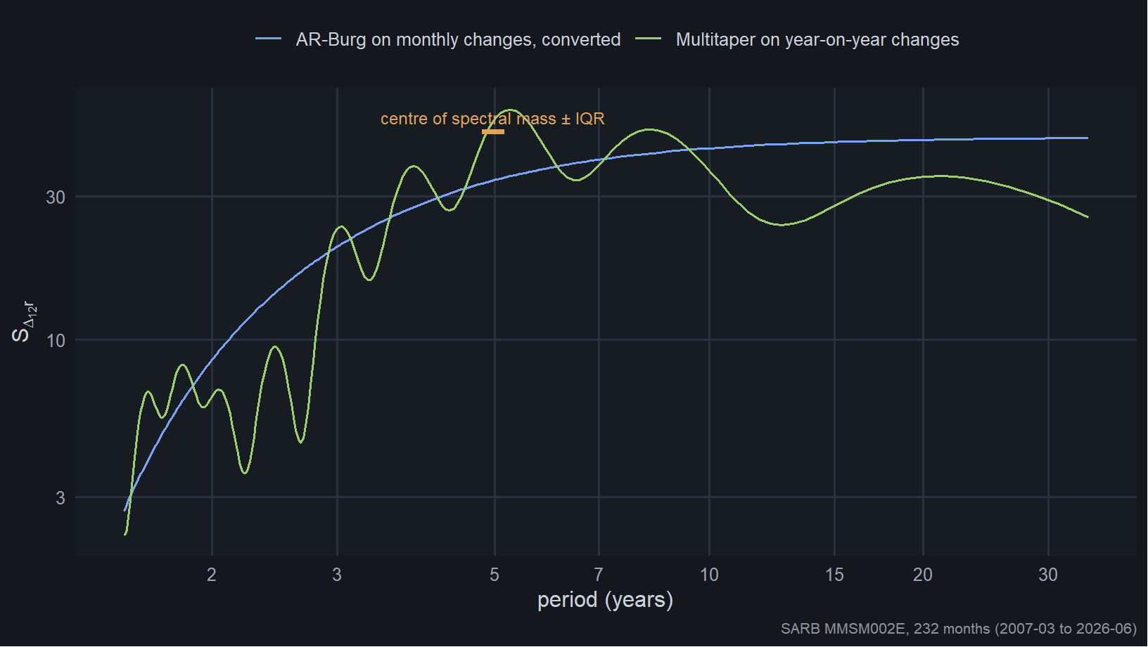
The line rises and flattens. Notice which moves dominate: the biggest ones Ire also the slowest, unfolding over three to four years, and slow large moves put their energy at long periods. That is why the curve climbs to the right and stays there.
The sample is 232 months, which sounds generous until you divide by the length of a rate cycle. Against a seventy-eight month cycle that is 3.0 realisations, and the resolution limit at that period is plus or minus 26 months - a five-and-a-half year cycle and a seven year cycle sit in the same bin. Anything I say about the height of a spectral feature here is decoration.
But the shape is not ambiguous, and the peak-finder’s failure is not a resolution problem. 93% of bootstrap replicates pinned the peak to the edge of the search range, which is what an algorithm does when asked to find something that is not there.
The caterpillar’s nulls point at nothing
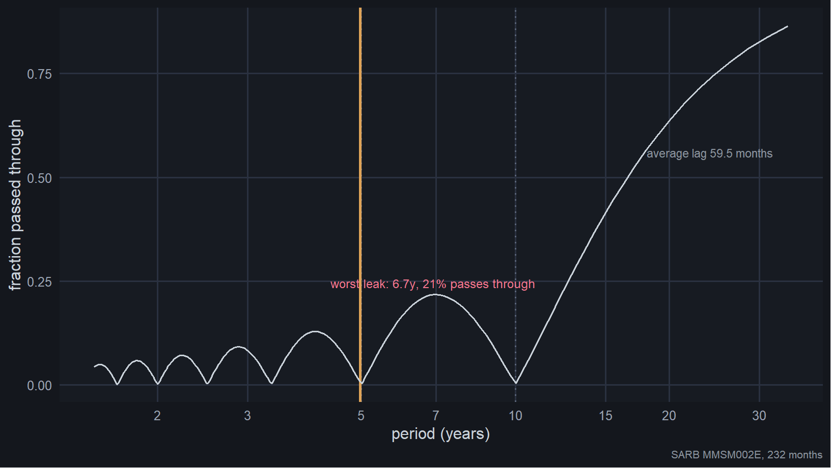
What that chart plots is the transfer function - the fraction of a rate wobble at each speed that survives the averaging. For a uniform ladder of $N$ months it has a closed form, the Dirichlet kernel:
$$H(\omega) = \frac{1}{N}\sum_{k=0}^{N-1} e^{-i\omega k} = e^{-i\omega (N-1)/2} \cdot \frac{\sin(N\omega/2)}{N \sin(\omega/2)}$$Here $\omega$ is angular frequency in radians per month, so a wobble with a period of $P$ months has $\omega = 2\pi/P$. The chart shows the magnitude, $|H(\omega)|$, which is the fraction passed through. The exponential in front is pure phase: its slope is exactly the $(N-1)/2$ month lag from before, which is why a moving average delays without distorting.
The magnitude vanishes wherever $\sin(N\omega/2) = 0$ but $\sin(\omega/2) \ne 0$, which happens when $N\omega/2 = \pi j$ - that is, at periods of $N/j$ months for $j = 1, 2, 3, \dots$ For $N = 120$ those are 120 months, 60 months, 40 months and so on: ten years, five years, three and a third. The nulls are not chosen. They fall out of the length.
The centre of spectral mass is at 5.0 years. The caterpillar has a null at five years. It is aimed almost perfectly.
Its aim was never the problem. The problem is everything to the right of that chart, where a ten-year average simply cannot reach: at a twenty-year period the filter passes about two-thirds of the variation straight through, and that is where South Africa’s rate moves actually live. The leaky side lobes that make the boxcar an embarrassment in a signal processing course turn out to be irrelevant here.
The hedge is shorter than the swaps you booked
Here is the part the textbook version of this analysis gets wrong, and it is not a rounding detail.
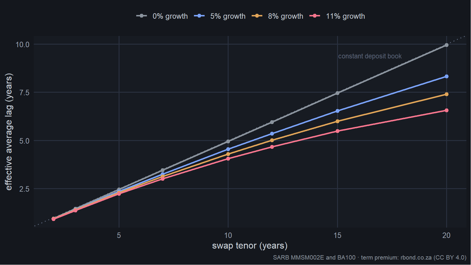
The standard treatment - ours included, until I checked - assumes a constant deposit base: roll one hundred and twentieth each month, hold one vintage of every age, weight them equally. Real programmes maintain notional as a percentage of a book that grows. Each month the desk books replacement tranches for what matured plus growth tranches for the larger base. And older tranches shrink as a share of today’s book, simply because today’s book is bigger.
So the weights are not equal. A tranche booked $k$ months ago was sized against a book that was smaller then, by a factor $e^{-ak}$ where $a = g/12$ is the monthly growth rate. As a share of today’s balance it has shrunk by exactly that much, so
$$h_k = \frac{e^{-ak}}{\sum_{j=0}^{L-1} e^{-aj}} \qquad\text{for } k < L, \qquad a = g/12$$The boxcar becomes a truncated exponential. Setting $g = 0$ recovers $h_k = 1/L$ and the textbook case, which is a useful check.
The average lag has a closed form too, and it is worth writing down because it shows exactly where the compression comes from:
$$\bar{k} = \frac{1}{e^{a}-1} - \frac{L}{e^{aL}-1}$$The first term is the lag you would get from an infinitely long programme on a growing book - about $1/a$ months, or twelve and a half years at 8% growth. It is a ceiling that growth alone imposes, with no reference to the swaps at all. The second term is the correction for actually stopping at $L$. At short tenors the second term dominates and the programme behaves as advertised; at long tenors it fades and the first term takes over. Past a certain point you are no longer buying lag from the swap market - you are bumping against a ceiling set by how fast your own deposit book grows.
I measured the growth rather than assuming it. BA100 core deposits for the total SA banking sector grew at 8.07% a year between 2013 and 2025, on the same definition the balance-sheet ratios in this post use. M3’s rolling twenty-year windows since 2000 sit between 8.8% and 11.1%. The scenarios below bracket both, so the 11% case is not a stress - it is the upper half of the plausible range.
| Swap tenor | no growth | 5% growth | 8% growth | 11% growth |
|---|---|---|---|---|
| 2 years | 1.0y | 0.9y | 0.9y | 0.9y |
| 3 years | 1.5y | 1.4y | 1.4y | 1.4y |
| 5 years | 2.5y | 2.4y | 2.3y | 2.2y |
| 7 years | 3.5y | 3.3y | 3.1y | 3.0y |
| 10 years | 5.0y | 4.5y | 4.3y | 4.1y |
| 12 years | 6.0y | 5.4y | 5.0y | 4.7y |
| 15 years | 7.5y | 6.5y | 6.0y | 5.5y |
| 20 years | 10.0y | 8.3y | 7.4y | 6.6y |
Table 1: Effective average lag. A twenty-year programme on a book growing at the rate I measured behaves like a seven-and-a-half-year one; at 11% it behaves like six and a half.
A twenty-year programme on a book growing 11% behaves like a 6.6-year one. The hedge you think you have is roughly two-thirds of the hedge you booked, and the gap widens with tenor.
What actually works: size it properly
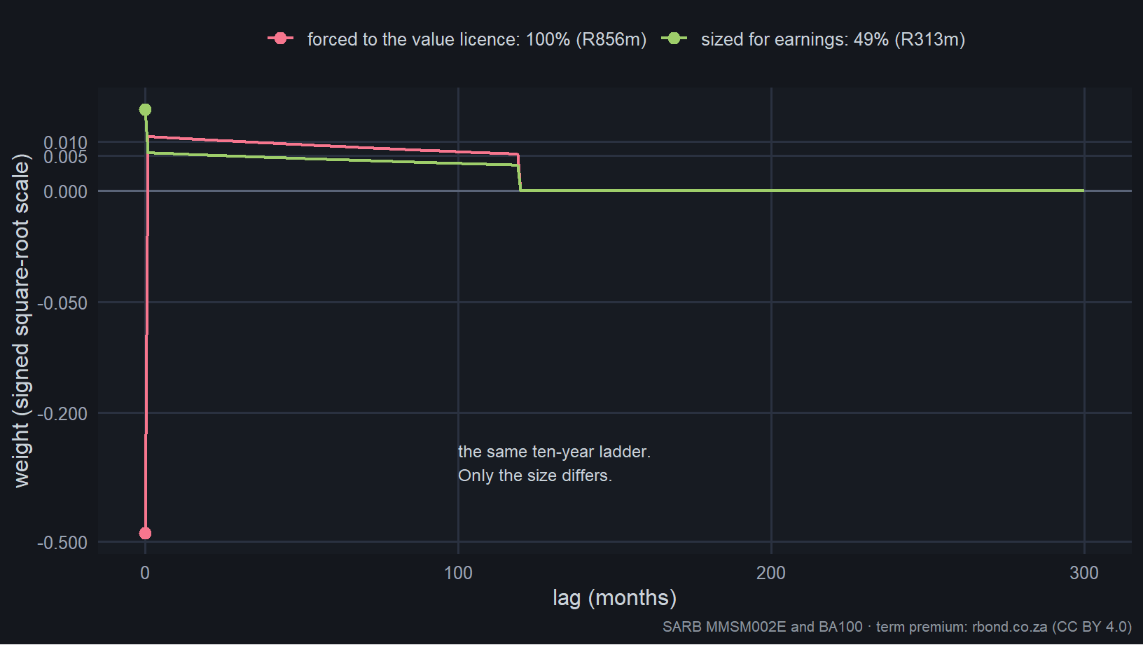
Post 2 priced the deposit franchise at 5.12 years of duration per rand of non-maturing deposits. Meeting that with ten-year swaps requires R126bn of notional against a R100bn deposit book. Nobody runs a 126% hedge ratio. Typical structural hedge ratios are 40–70% of non-maturing balances - and, as it turns out, that is almost exactly what the earnings objective wants.
Why the size matters more than anything else
What ALCO actually cares about is not the hedge’s own income but net interest income, and writing that down explains the whole post. Per rand of non-maturing deposits, with $N$ the notional and $h_k$ the ladder’s weights:
$$\Delta_{12}\text{NII}_t = (1 - \beta - N)\,\Delta_{12}r_t + N\sum_{k \ge 1} h_k\,\Delta_{12}r_{t-k}$$The first term is today: the bank gains $(1-\beta)$ per rand from the deposit book repricing and pays $N$ per rand on the swap’s floating leg. The second is the fixed leg, which is still earning rates struck up to $L$ months ago. Writing the whole thing as one filter $h^{\text{net}}$, its coefficients have a property that does not depend on the ladder at all:
$$\sum_k h^{\text{net}}_k = (1 - \beta - N) + N\sum_k h_k = (1-\beta) - N + N = 1-\beta$$A structural hedge cannot remove rate exposure from earnings. It can only move that exposure to different frequencies. Whatever the programme, the bank’s sensitivity to a permanent shift in rates is the same $1-\beta$ it always was. Only the timing changes.
Now the objective. The variance of that year-on-year change is a quadratic form in the weights:
$$\mathcal{V}(h^{\text{net}}) = \sum_j \sum_k h^{\text{net}}_j h^{\text{net}}_k \, \gamma(|j-k|) \qquad\text{where}\qquad \gamma(d) = \text{Cov}\!\left(\Delta_{12}r_t,\, \Delta_{12}r_{t-d}\right)$$and $\gamma$ is exactly what the spectrum estimated. Differentiating with respect to $N$ and setting it to zero gives the optimal size in closed form. Writing $u = h - e_0$ for the difference between the ladder’s weights and a spike at lag zero:
$$N^{\star} = (1-\beta)\,\frac{\gamma(0) - \sum_k h_k\gamma(k)}{\gamma(0) - 2\sum_k h_k\gamma(k) + \sum_j\sum_k h_jh_k\gamma(|j-k|)}$$That looks worse than it is. For a long, smooth ladder the averaging kills almost all of the variance, so the sums involving $h$ shrink toward zero and the whole fraction tends to one:
$$N^{\star} \longrightarrow 1 - \beta$$That is the sizing rule, and it is why the answer came out between 40% and 51% rather than at exactly 51.1%. The correction terms are small but not zero, and they shrink as the ladder lengthens - which is why the optimal size creeps upward with tenor in the table below. Practice sets the hedge ratio somewhere in a 40–70% band by convention; this says the number is one minus the deposit beta, and says why.
The dipole was a sizing mistake, not a tenor one. What is happening is easy to see on the day of a hike. With R100bn of ten-year swaps, the bank pays an extra R1,000m on the floating leg while the fixed leg sits unchanged, against the R511m it gained on the deposit book: net −R489m. The hedge did not damp the exposure, it overshot and flipped the sign. Sized at 49% instead, the floating leg costs about R490m against that R511m and the two very nearly cancel - which is the whole idea.
Every tenor, at its own best size
So ask the fair question instead: what does each horizon deliver at its own best size? Horizons stop at twenty years here, because most treasuries will not transact beyond that in size, and the results say they need not.
| Programme | best size | income per year | volatility | volatility cut | % of value licence |
|---|---|---|---|---|---|
| no hedge at all | — | R0m | R828m | — | 0% |
| 2 years | 41% | R42m | R600m | 27% | 8% |
| 3 years | 43% | R136m | R518m | 37% | 13% |
| 5 years | 46% | R410m | R422m | 49% | 22% |
| 7 years | 48% | R677m | R365m | 56% | 31% |
| 10 years | 49% | R1083m | R313m | 62% | 43% |
| 12 years | 50% | R1268m | R290m | 65% | 51% |
| 15 years | 50% | R1539m | R264m | 68% | 62% |
| 20 years | 51% | R1718m | R237m | 71% | 79% |
Table 2: Per R100bn of non-maturing deposits, on a book growing 8% a year. Income is the term premium the programme earns; volatility is the standard deviation of the year-on-year change in net interest income. The last column is how much of Post 2’s value-based duration licence the programme covers - and it never reaches 100%.
A ten-year caterpillar at a 49% hedge ratio cuts earnings volatility by 62% and earns R1083m a year. It is a perfectly good hedge. Even a five-year programme roughly halves the volatility. There is no tenor at which hedging fails to help.
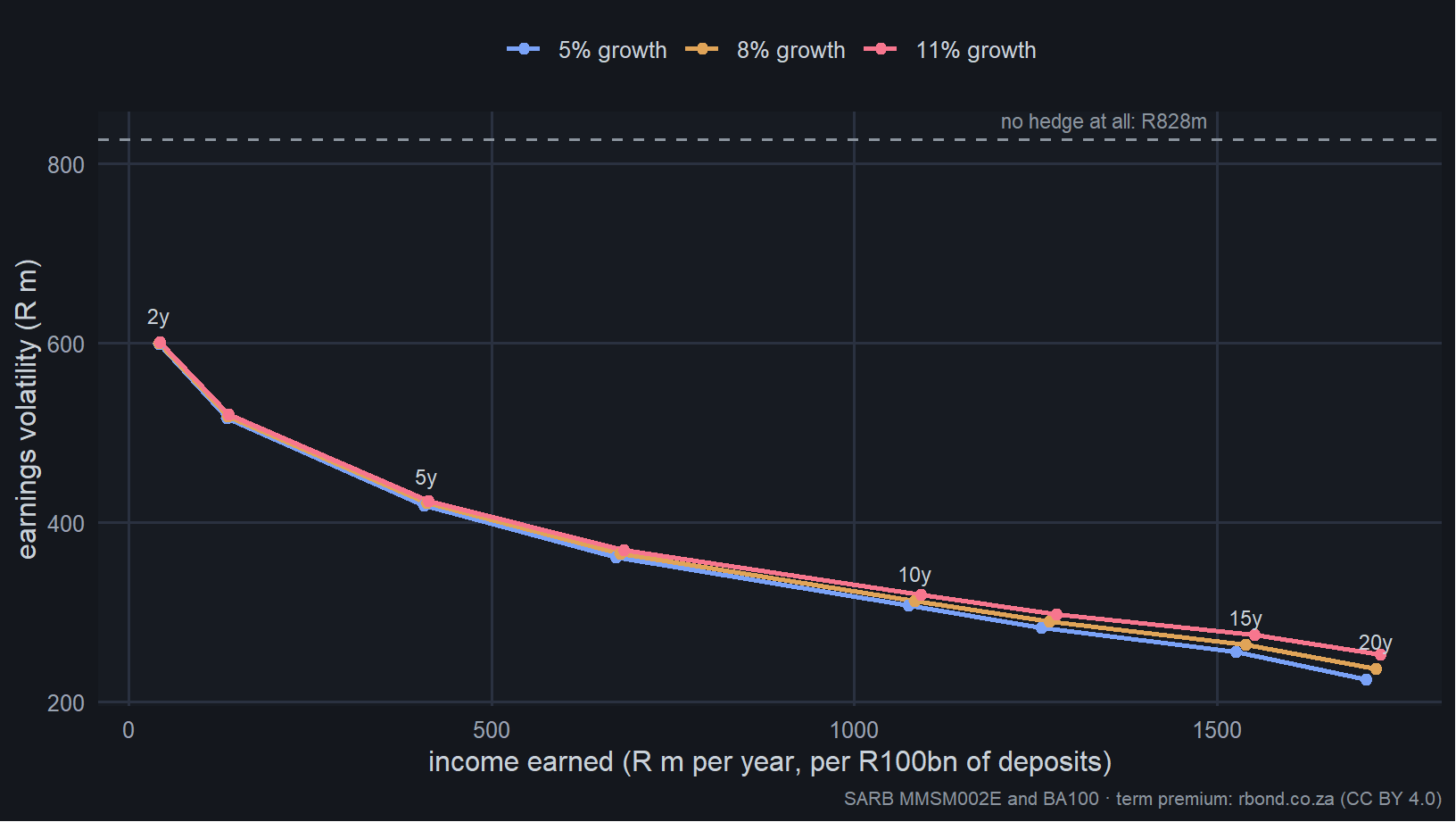
Two things stand out, and both are more useful than anything the filter theory produced.
The best hedge ratio is 40–51% across every tenor and every growth rate tested. It is tracking $1-\beta = 0.511$, and it barely moves. That is a robust operating rule and the single most valuable number in this post.
And the three growth curves nearly overlap. Growth shifts income and volatility by only a few per cent, because the size decision dominates the shape decision. Growth matters enormously for what the programme is - a twenty-year ladder is really a seven-year one - and hardly at all for what it delivers, once it is sized correctly.
The last column of the table is the uncomfortable one. Even a twenty-year programme at its own best size reaches only 79% of the value licence. Sizing for earnings leaves value risk on the table, and nothing in the tradeable tenor range closes the gap. That is the genuine tension: not that hedging is bad, but that the earnings objective and the value objective want different-sized books, and no ladder satisfies both.
Filter shaping buys nothing
Now solve the whole thing properly. Minimise earnings volatility over every combination of roll flows across every tenor, with growth in the mechanics, subject to the notional cap. It is a convex quadratic program and it solves in milliseconds.
The answer is a single tenor at the longest horizon available, and the gain over simply picking that tenor is 0.00 bps, at every growth rate tested.
The reason follows from the tail-sum identity at the top. Because $h_k = \sum_{m>k} c_m$ with every $c_m \ge 0$, the weights must satisfy
$$h_0 \ge h_1 \ge h_2 \ge \dots \ge h_{L-1} \ge 0$$and conversely any such sequence can be built by choosing $c_m = h_{m-1} - h_m$. So the set of programmes a spot ladder can construct is exactly the set of non-increasing weightings - no more, no less.
Now ask which member of that set minimises the objective. Concentrating weight raises the quadratic form; spreading it lowers it. The clean case is white noise, where $\gamma(d) = 0$ for $d \ne 0$ and the variance collapses to $\gamma(0)\sum_k h_k^2$ - and for a fixed total $\sum_k h_k$ over a fixed support, $\sum_k h_k^2$ is minimised by making every weight equal. That is the uniform ladder. Rates are not white noise, so this is an argument rather than a proof, and I checked it numerically instead: across every tenor and growth rate tested, the optimiser returned the uniform ladder to two decimal places. Flattest means most smoothing, which is exactly what the objective rewards. RBS did not pick the uniform caterpillar by luck. It is the best member of its own family, and a decade of desks copying it Ire not being lazy.
That leaves forward-starting swaps, the one way out of the declining family, since they weight a block of past rates while ignoring the most recent ones. They Ire tested rather than assumed, and they lose twice. On duration: counting notional from trade date, as a notional register does, a swap starting in two years and running ten occupies the same twelve years of footprint as a spot twelve-year swap but earns less duration, because the waiting period contributes nothing. On the objective: offered the full menu, the optimiser gave them zero weight at every delay.
Could I not time the cycle?
The obvious next thought, and the one every ALCO raises: hedge more when rates are high, less when they are low. Lock in the peaks. I tested it by simulating rate paths with the estimated spectrum and running timing rules against a static programme.
| Rule | income | volatility | beats static on both |
|---|---|---|---|
| static, no timing | R1,701m | 1.0× | — |
| timed on the rate level, mild | R1,837m | 2.0× | 0% |
| timed on the rate level, aggressive | R2,157m | 3.5× | 0% |
| perfect foresight | R3,003m | 2.0× | 0% |
Even knowing the next two years of rates exactly, timing never improved both. Not rarely - never, across two hundred simulated paths.
There is a mechanical reason and it is the useful part. The floating leg costs notional × rate. Hold notional fixed and that is a constant times a moving quantity. Let notional vary and it becomes a product of two moving quantities, which is strictly more variable. Timing buys income at a guaranteed volatility cost, paid whether or not the forecast is any good. Perfect foresight earned R1.3bn more and still doubled the volatility.
And the signals are not there anyway. Cycle position is dead already - there is no cycle to be early or late in. Rate level is dead by a number already in this post: the model fits the monthly changes as stationary, which makes the level a random walk, and a random walk’s current level tells you nothing about the direction of its next move. Curve slope is the one with real literature behind it, and the Cochrane–Piazzesi finding that the predictable term premium does not survive out of sample is the reason to keep expectations modest.
A different instrument entirely
All of the above assumes swaps. It need not. The same duration can be bought by taking the deposits and buying fixed-rate government bonds - which is what a great many banks in fact do - and in South Africa the two are not priced the same.
SA government bonds yield materially more than the matched swap. The gap is measured directly from the overlap in the data behind this post: 57bp at one year, widening to 156bp at ten years and held flat beyond, which is the convention the SARB’s own derivatives workstream uses for the equivalent spread. A bank that buys the bond rather than receiving fixed on the swap collects that on every rand, for identical duration and therefore identical earnings volatility.
| Route | income per year | volatility | what you take on |
|---|---|---|---|
| receive fixed on swaps | R1718m | R237m | collateralised, off balance sheet, hedge-accountable |
| buy government bonds | R2506m | R237m | consumes balance sheet; marks flow through to capital |
Table 3: A twenty-year programme at 51% of a R100bn deposit book, built two ways. Same duration, same earnings volatility. The bond route earns R787m a year more - which is payment for risks the swap does not carry, not a free lunch.
That is the largest number in this post and it deserves care rather than celebration. The spread is compensation for real risks the swap does not carry, and three of them matter.
Sovereign credit. A swap is collateralised daily against a bank counterparty. A government bond is an unsecured claim on a sub-investment-grade sovereign. A good deal of that 156bp is simply the price of that, and anyone who has spent a Friday evening waiting on a ratings announcement knows why it is not small.
Capital volatility, which is the one that ends careers. Bonds held at fair value mark to market, and those marks flow through to capital. A twenty-year bond portfolio at half the deposit base would swing capital hard as rates move - which is precisely what happened to several US banks in 2023. A swap designated as a cash flow hedge does not do that. So the bond route delivers identical earnings stability while giving up capital stability. Those are different balance sheets in a stress.
Balance sheet capacity. Bonds consume leverage-ratio headroom even where they attract no credit risk weight, and that headroom has an internal price no public dataset can tell you.
Note the coupling, because it changes the tenor answer. Bond capital volatility scales with duration, so a bank taking the R787m should think about a shorter book than the swap analysis alone would suggest. The instrument decision and the tenor decision are not independent.
So what should the desk do?
| # | Decision | What the analysis says | Worth |
|---|---|---|---|
| 1 | Which instrument | Bonds pay 156bp over matched swaps at ten years and beyond, for identical rate risk. Take it only if the balance sheet and the capital-volatility appetite are there. | R787m a year |
| 2 | How big | About 49% of the non-maturing book. That is one minus beta, and it holds across every tenor and growth rate tested. | R515m of volatility removed |
| 3 | How long | Longer is better on both axes, but growth eats the benefit past fifteen years. Ten to fifteen captures most of it. | R158m more, 5y to 15y |
| 4 | What shape | Uniform. Do not build a weighting scheme. | R0m |
| 5 | Whether to time it | No. Even perfect foresight fails. | negative |
Table 4: In descending order of what each is worth, per R100bn of non-maturing deposits per year.
As a single instruction: run about half your non-maturing deposit base in a uniform ladder of ten to fifteen years, and have a serious argument about whether it should be bonds rather than swaps. Nothing in that requires a spectrum, a filter or a quadratic program - but it took all three to be confident that nothing more elaborate was being left on the table.
What would change it. Decision 1 reverses if capital volatility is scarce. Decision 2 tightens if the economic-value limit binds before the earnings objective does. Decision 3 is capped by what actually trades, and by how fast the book is growing. Decision 4 did not reverse under anything I tested, including the full forward-start menu.
The ALCO bridge
| Bridge leg | R m on R100bn | bps of NIM | bps of pre-tax ROE |
|---|---|---|---|
| 5-year programme at its best size | R422m | 16.2 | 200 |
| extend to 10 years | -R109m | -4.2 | -52 |
| extend to 15 years | -R49m | -1.9 | -23 |
| optimise the filter shape | R0m | 0.0 | 0 |
| optimised programme | R264m | 10.2 | 126 |
| memo: no structural hedge at all | R828m | 31.8 | 393 |
Table 5: Year-on-year NII volatility. Balance-sheet ratios are averages over 36 monthly BA100 returns for the total banking sector: core deposits are 68.3% of interest-earning assets, and interest-earning assets are 12.4 times ordinary equity. Tax is omitted deliberately - it is a uniform scalar that cannot change any ranking - so the ROE column is pre-tax.
Because a bank holds roughly one rand of capital for every 12.4 of assets, a small move in margin becomes a large move in return on equity. One basis point of NII per rand of the non-maturing deposit base is 0.385 bps of net interest margin and 4.75 bps of pre-tax return on equity. The whole bridge from a five-year to a fifteen-year programme is 75 bps of pre-tax ROE volatility, and the fourth line - reshaping - is zero.
What this is not
The sample is 232 months - three realisations of a rate cycle - so what I say about where spectral mass sits is on firmer ground than anything about how much. The term premium is measured over a window that includes the 2020 steepening and therefore flatters itself. Growth is treated as a constant when it demonstrably is not, as above.
The optimisation always wants the longest tenor available, so whether twenty-year rand swaps trade in the size a structural hedge needs is a question for a desk rather than a spectrum. Growth makes that question less urgent than it looks: the gap between a fifteen-year and a twenty-year programme is small once the book is growing, so a treasury that cannot go past fifteen is giving up very little.
Finally, this post measures earnings volatility throughout. Post 2’s licence is about economic value. A committee managing to earnings and one managing to value will read the same ladder differently, and the gap between them - 79% at best - is the number to put on the slide rather than any single ladder.
Basel Committee on Banking Supervision. 2016. Interest Rate Risk in the Banking Book. Standards No. d368. Bank for International Settlements. https://www.bis.org/bcbs/publ/d368.htm.
Cochrane, John H., and Monika Piazzesi. 2005. “Bond Risk Premia.” American Economic Review 95 (1): 138–60. https://doi.org/10.1257/0002828053828581.
Drechsler, Itamar, Alexi Savov, and Philipp Schnabl. 2021. “Banking on Deposits: Maturity Transformation Without Interest Rate Risk.” The Journal of Finance 76 (3): 1091–143. https://doi.org/10.1111/jofi.13013.
Percival, Donald B., and Andrew T. Walden. 1993. Spectral Analysis for Physical Applications: Multitaper and Conventional Univariate Techniques. Cambridge University Press. https://doi.org/10.1017/CBO9780511622762.
South African Reserve Bank. 2023. Market Conventions for ZARONIA-Based Derivatives. Market Practitioners Group, Derivatives Workstream. https://www.resbank.co.za/content/dam/sarb/publications/media-releases/2023/zaronia-based-derivatives/Market\20conventions\20for\20ZARONIA-based\20derivatives.pdf.
South African Reserve Bank. 2025. Historical Estimation of the ZARONIA OIS Curve. Market Practitioners Group, Derivatives Workstream. https://www.resbank.co.za/en/home/publications/publication-detail-pages/Financial-Markets/Committees/MPG/MPG-Related-pages/2025/historical-estimation-of-the-zaronia-ois-curve.