The Price of Not Knowing
Three posts ago this series set out to model South African deposits properly, on the theory that a bank which understands its own funding can price it better than one which does not. The theory survived. What did not survive was my expectation about where the interesting risk would turn out to be.
In post 1 I built a hierarchical state-space model of deposit behaviour and found that balances are random-walk-permanent. They do not run off. They drift. The useful half of that post was what the model recovered along the way. Pass-through betas separate cleanly by product, from 0.24 on term money up to 0.62 on notice deposits, and pricing the whole book off a single flat beta misstates its economic value by 32.5 basis points of the deposit base, which is about 3.2% of CET1. Letting those betas move instead of resetting them once a year was worth 12 basis points of return on equity, recurring.
Post 2 differentiated a franchise valuation simulator and found the warranted behavioural haircut on duration is zero, because the smooth rate-chasing channel is inert. It also put a number on the thing the haircut was meant to modify, in the franchise-duration framing of Drechsler et al. (2021). The deposit franchise licenses 5.12 years of maturity transformation per rand of non-maturing base, and measured going-concern rather than as a runoff of the existing cohort the duration is -7.3 years against -1.0. Those are not the same balance sheet, and the second one is what most banks are looking at.
In post 3 I rebuilt the structural hedge as a finite-impulse-response filter, optimised the ladder shape against the estimated rate spectrum, and beat the incumbent boxcar by 0.00 basis points. Shape does nothing at all. Size and tenor do nearly everything: the optimal notional converges on 49% of the book, which is one minus the pass-through beta on non-maturing deposits and therefore a quantity you can derive rather than negotiate, and running it cuts year-on-year earnings volatility by 62%. Stretching the programme from ten years to twenty lifts the share of Post 2’s licence you actually capture from 43% to 79%.
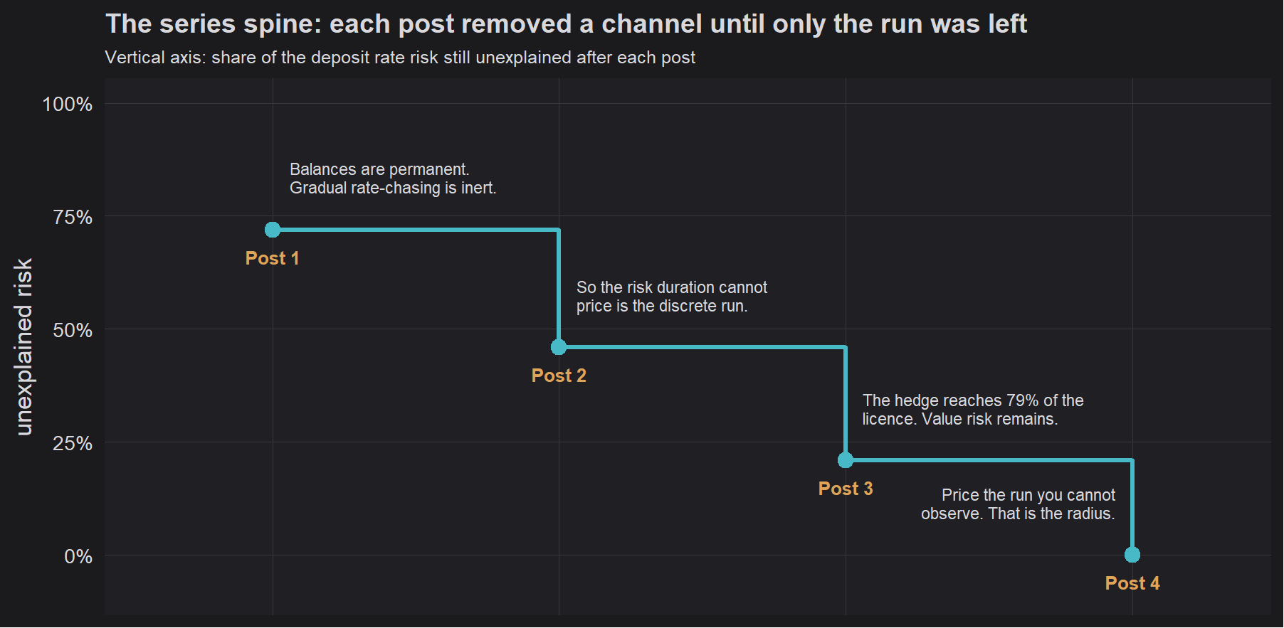
Read as a sequence that is either a catastrophe or a fascinating result. Each post removed a candidate explanation for deposit rate risk and left the residual smaller and sharper. By the end of Post 3 the residual had a name - the discrete run - and one property that made it untouchable: it is invisible in the public dataset this series uses.
The thing that has been missing all along
Every post in this series has walked into the same wall. Each time I dropped it into the “What didn’t work” section.
Post 1 tested whether competitive flows between banks respond to rate movements at monthly frequency and got a clean null. Part of that was share-shifts differencing out the level. The rest was the data itself: BA 900 (South African Reserve Bank 2025) records net movements, so money arriving and money leaving are added together before anyone outside the bank sees a number.
Post 2 computed the behavioural haircut on franchise duration and got zero. Some of that was a real finding, because SA balances genuinely are permanent. But the caveat was identical. A net series cannot show you customers leaving while other customers arrive, so the estimated churn is a lower bound of unknown tightness.
Post 3 sized the structural hedge for earnings and found that even a twenty-year programme at its best size reaches only 79% of the value licence Post 2 computed. The gap is value risk, and no tradeable swap tenor closes it.
Three methods, three questions, same single blind spot.
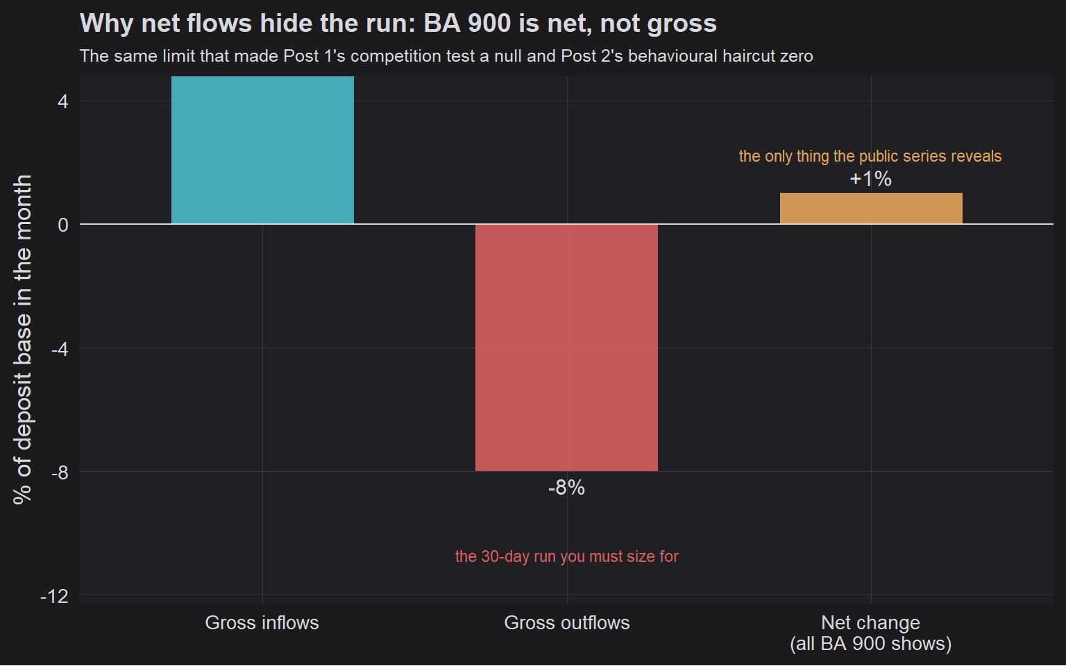
A bank run is a coordination failure, not a slow drift (Diamond and Dybvig 1983), and it does not arrive as a tidy negative number in an aggregate monthly return. It does not fill in a form and it does not take a queue ticket. It arrives as an enormous gross outflow which may, in the same month, be partly papered over by deposits fleeing towards you from somewhere worse. The published series is structurally incapable of showing it. That is not a complaint about data quality. The returns are doing precisely the job they were designed to do. It is a statement about the limits of what anyone standing outside a bank can know.
Which gives the finale a specific job. Price a risk that cannot be estimated. Estimating and pricing are different problems, and only the second one is something I can post about on a public blog.
Sizing a buffer, and the usual two bad ways to do it
A bank holds high-quality liquid assets so that when depositors want their money back at once, it can oblige. HQLA earns roughly the repo rate. The same rand lent out earns considerably more. So the buffer is a tax on the possibility of a bad month, and the only real question is how large that tax should be.
The regulator’s answer is the LCR (Basel Committee on Banking Supervision 2013). Multiply each deposit category by a prescribed runoff weight, add up, hold at least that much. This is fine in the way a speed limit is fine. It is a number chosen by committee to be safe for everybody and therefore exactly right for nobody, and it commands roughly the same respect South Africans extend to the 120 sign on the N1.
The industry’s other answer is to pick a stress scenario and size to survive it. In practice this means choosing whichever apocalypse the risk team found most compelling after a particularly motivating offsite, then assuming the remaining apocalypses have agreed to hold off. They have not agreed to anything. Nobody asked them. It is the risk-management equivalent of the load-shedding schedule: published in advance, formatted beautifully, and only loosely related to what happens at half past six.
What you actually want is to survive all the plausible bad months at once, with plausible defined honestly rather than by whoever presented last. That is a solved problem, and its solution is where the run finally gets a price.
The ball, formally
Start with the cost of being wrong. On the space of possible monthly outflows, the cost of moving a unit of probability mass from level $\xi$ to level $\xi'$ is the distance $\lVert\xi-\xi'\rVert$ between them. Your data is $N$ pooled bank-months, treated as a distribution built from point masses, one grain of sand of weight $1/N$ at each observed month:
$$\hat{\mathbb{P}}_N \;=\; \frac{1}{N}\sum_{i=1}^N \delta_{\xi_i}.$$The type-1 Wasserstein distance between that pile and any candidate distribution $\mathbb{Q}$ is the cheapest way to shovel one into the other (Villani 2009):
$$W_1\big(\hat{\mathbb{P}}_N,\mathbb{Q}\big) \;=\; \inf_{\pi\,\in\,\Pi(\hat{\mathbb{P}}_N,\,\mathbb{Q})} \int \lVert \xi - \xi' \rVert \,\mathrm{d}\pi(\xi,\xi'),$$where $\Pi(\hat{\mathbb{P}}_N,\mathbb{Q})$ is the set of transport plans, meaning joint distributions whose margins are $\hat{\mathbb{P}}_N$ and $\mathbb{Q}$. The plan says how much mass travels from each $\xi$ to each $\xi'$. You pay distance times mass and keep the cheapest plan going, which is the only setting in which hiring a TLB by the hour counts as a rigorous mathematical operation. The ambiguity set is then just a ball in that metric:
$$\mathbb{B}_\varepsilon(\hat{\mathbb{P}}_N) \;=\; \big\{\, \mathbb{Q} : W_1(\hat{\mathbb{P}}_N,\mathbb{Q}) \le \varepsilon \,\big\}.$$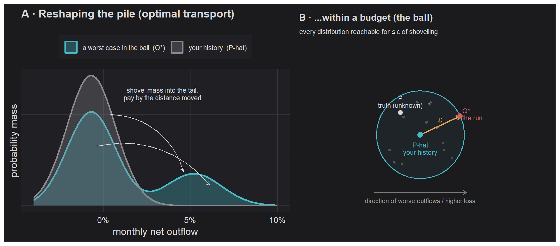
Two properties make this the right object for the task rather than merely a fashionable one.
It can put mass where you have never been. The adversary is allowed to drag a grain of sand out into a tail fatter than anything in your history, which is exactly what is required when net flows cannot see a gross run. A ball built on Kullback-Leibler divergence cannot do this, because KL is infinite against any distribution whose support escapes your sample. It can only reshuffle the disasters you have already lived through, which rather misses the point of worrying about new ones.
The radius is not a mood. The empirical distribution converges to the truth in Wasserstein distance at a known rate. Fournier and Guillin (2015) give $\mathbb{E}\,W_1(\hat{\mathbb{P}}_N,\mathbb{P}) \lesssim N^{-1/\max(d,2)}$, so for confidence $\beta$ you can pick $\varepsilon_N(\beta)$ such that the unknown true distribution lies inside the ball with probability at least $1-\beta$. “How paranoid are we” becomes “how much should we distrust a finite sample”, and that is a question with an actual answer.
From ball to buffer
Let $\xi$ be the 30-day net outflow as a fraction of deposits, $B$ the buffer, and the carry $(r_{\text{deploy}}-r_{\text{HQLA}})\,B$. The problem is
$$\min_{B\ge 0}\ (r_{\text{deploy}}-r_{\text{HQLA}})\,B \quad\text{s.t.}\quad \sup_{Q\in\mathbb{B}_\varepsilon(\hat{\mathbb{P}}_N)}\ \mathrm{CVaR}_\alpha^{\,Q}\!\big(\xi - B\big)\ \le\ 0,$$with $\mathrm{CVaR}_\alpha$ the average outflow in the worst $1-\alpha$ of months, the coherent tail measure of Artzner et al. (1999). Not the single worst case, since the genuine worst case in banking is always “slightly worse than whatever you put in the model”, a quantity with much the same forecasting record as the winter outlook, but the average of the bad days, which is at least estimable.
The inner problem maximises expected loss over every distribution in the ball, an infinite-dimensional optimisation over measures. Mohajerin Esfahani and Kuhn (2018) and Gao and Kleywegt (2023) show the Lagrangian dual collapses it to one dimension, and Blanchet and Murthy (2019) give the same result in a model-risk framing:
$$\sup_{\mathbb{Q}\in\mathbb{B}_\varepsilon}\ \mathbb{E}_{\mathbb{Q}}[\ell(\xi)] \;=\; \inf_{\lambda\ge 0}\ \Big\{\, \lambda\varepsilon \;+\; \tfrac{1}{N}\sum_{i=1}^N \sup_{\zeta}\big[\,\ell(\zeta) - \lambda\lVert \zeta - \xi_i \rVert\,\big] \Big\}.$$Read the parts. $\lambda$ is the shadow price of the transport budget. The inner supremum is the adversary dragging each observation to a nastier value and being charged $\lambda$ per unit of distance. If the loss climbs no faster than slope $L$, the adversary pushes along that slope until the transport charge catches up, and the optimal price turns out to be exactly $\lambda = L$. Everything else cancels:
$$\sup_{\mathbb{Q}\in\mathbb{B}_\varepsilon}\ \mathbb{E}_{\mathbb{Q}}[\ell(\xi)] \;=\; \frac{1}{N}\sum_{i=1}^N \ell(\xi_i) \;+\; \varepsilon\,L.$$Now apply that to CVaR, where there is a factor waiting to catch you out.
CVaR is not itself a plain expectation, so you cannot read the Lipschitz constant off the outflow directly. You have to go through the Rockafellar-Uryasev representation (Rockafellar and Uryasev 2000, 2002), which turns CVaR into an ordinary expectation by minimising over a threshold $\tau$:
$$\mathrm{CVaR}_\alpha(Z) \;=\; \min_{\tau}\ \Big\{\, \tau + \tfrac{1}{1-\alpha}\,\mathbb{E}\big[(Z-\tau)^{+}\big] \Big\}.$$The function sitting inside that expectation is what the adversary actually attacks, and it has a $\tfrac{1}{1-\alpha}$ in front of it. At $\alpha = 0.975$ that factor is 40. So the loss the adversary faces is not 1-Lipschitz in the outflow. It is 40-Lipschitz, and the correct result is
$$\boxed{\,B^\star(\varepsilon)\ =\ \widehat{\mathrm{CVaR}}_\alpha(\xi)\ +\ \frac{\varepsilon}{1-\alpha}\,}$$The tempting shortcut is to write $B^\star(\varepsilon) = \widehat{\mathrm{CVaR}}_\alpha(\xi) + \varepsilon$, on the reasoning that outflows are measured in units of themselves so the Lipschitz constant must be one. That reasoning applies to an expectation, not to a CVaR, and the missing factor is not a rounding detail. At this confidence level it is 40. It is worth seeing why it is there rather than taking it on trust, because the intuition is simple once you have it.
Suppose the adversary has a shovelling budget of $\varepsilon$ and wants to make the worst 2.5% of months as bad as possible. Moving a large amount of mass a short way is inefficient, because most of that mass lands outside the tail where it does not affect CVaR at all. The efficient attack is the opposite: take a tiny sliver of probability, say a quarter of a percent, and hurl it an enormous distance. The budget is mass times distance, so a sliver of 0.25% can be moved 400 times further than a block of 100% for the same price. That sliver is guaranteed to land in the worst 2.5%, and once there it is averaged over the tail with weight $1/(1-\alpha)$. The adversary therefore converts every rand of transport budget into forty rands of CVaR.
Worth noting what the factor does and does not touch. Every buffer level in this post is computed somewhere other than this formula: the LCR requirement from multiplying deposits by runoff weights, the run-anchored buffer from multiplying the runnable base by a severity, the empirical CVaR straight from the data. The formula’s job is to translate between a buffer and a radius, so it sets the scale on which the four answers are compared rather than the answers themselves. Get it wrong and every buffer is still right while every comparison is quietly nonsense, which is a satisfying way for a model to fail in that it leaves no visible mess.
The whole thing is an LP with a one-dimensional dual and finite-sample guarantees attached, and once you have the CVaR it fits on the back of a Castle Lager coaster. For a method with “distributionally robust” in the name, that is almost suspicious.
NGFB’s actual book
Here the series starts paying for itself. The composition below was not invented for this post. It is Post 1’s canonical draw, a truncated posterior-predictive sample across the SA majors with bank effects integrated out.
Mapping that book onto the LCR runoff buckets throws up the first genuine surprise.
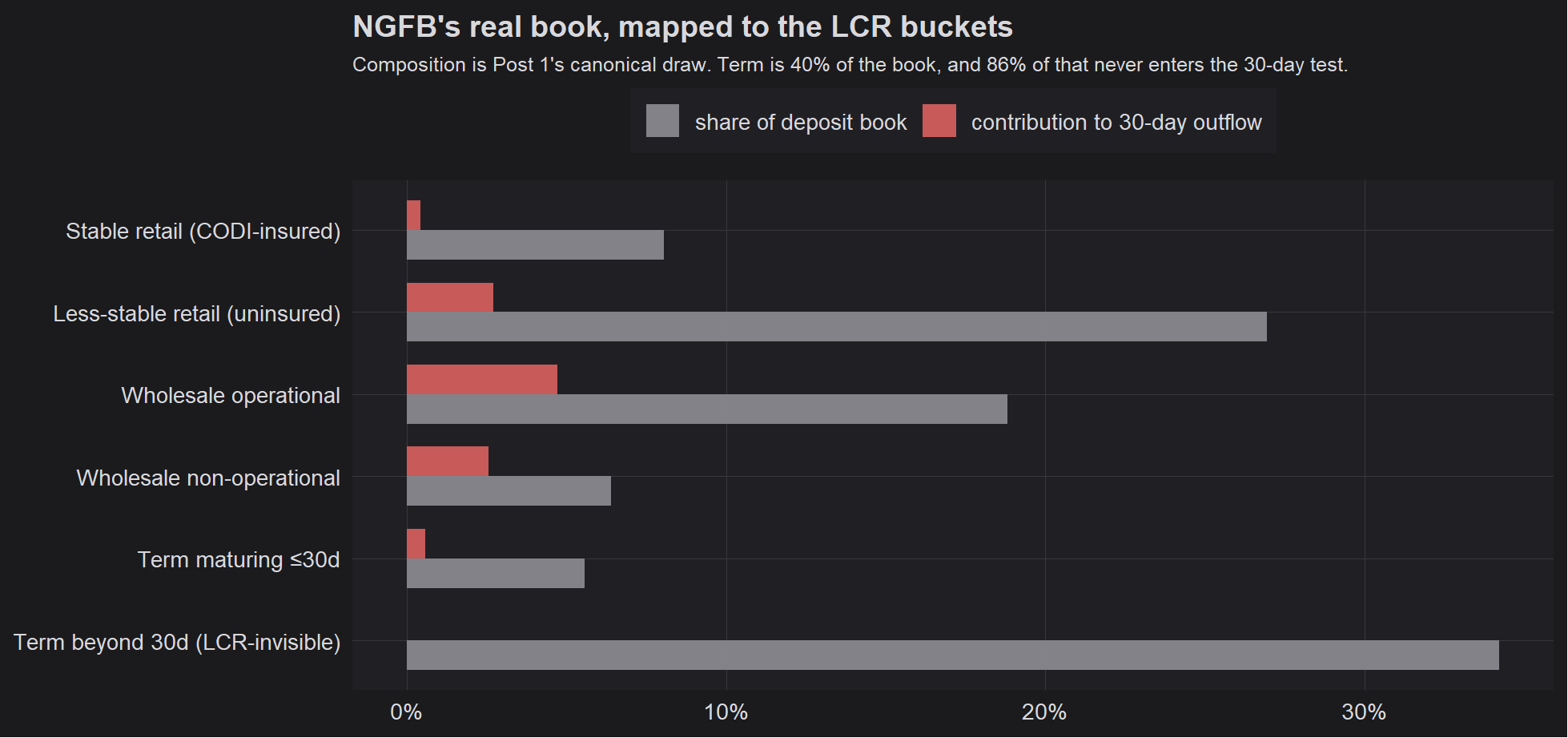
40% of NGFB’s book is term deposits, and the overwhelming majority of that matures beyond thirty days, so it contributes nothing whatsoever to the regulatory outflow. NGFB’s total regulatory NCO lands at 10.9% of deposits, and much of the reason it looks so comfortable is a structural quirk of South African bank funding rather than any prudence on NGFB’s part. The term book is not safe. It is simply invisible, which is an entirely different property that happens to look identical from where the compliance dashboard is standing. Much like a pothole at night, only the observation has been deferred.
The other structural fact arrives from Post 2’s axis. CODI has been operational since 1 April 2024, with cover of R100,000 per depositor per bank (South African Reserve Bank 2024a). That is a serious sum for most South Africans and about a fortnight of bond repayments in parts of Sandton, which is the entire problem compressed into one sentence. That protects roughly nine in ten depositors by headcount. But a small number of large balances dominate the rand value, so it insures only about 23% of deposits by value, leaving 77% of the base runnable in principle. That figure is not a modelling choice. It is arithmetic performed on a published policy parameter, and it is the most important input in this post.
The pooled distribution, and a quiet confirmation
The empirical measure at the centre of the ball is the pooled marginal, meaning the outflow distribution for a representative and deliberately unobserved bank drawn from the population, with individual bank effects integrated out. That construction is the series aggregation rule. It is simultaneously the correct statistics for a five-group panel and the reason nobody can reverse-engineer an institution from the chart.
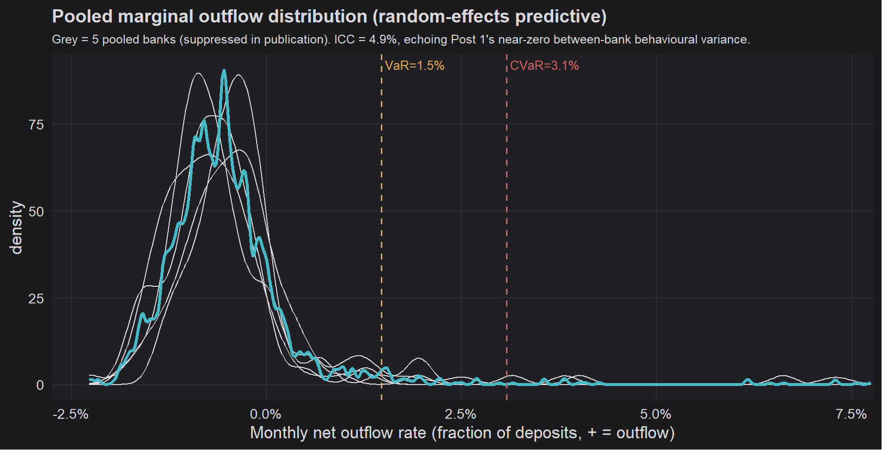
The variance decomposition puts the intraclass correlation at 4.9%. Almost all the variation in monthly deposit flows is a bank differing from its own past rather than from its peers. Post 1 arrived at the same conclusion down a completely different road, finding that between-bank behavioural variance pooled to approximately zero and that NGFB’s distinctiveness comes from what it holds rather than how it behaves. Two methods, two datasets, one answer. That is the closest this series will get to independent replication, and I value it more than any single headline number in it. It is also the only occasion in four posts on which two calculations have agreed without being asked to.
Four answers, on one scale
Each anchor below is a different answer to the question “how much should we distrust our own history”, expressed as a shovelling budget. Because the buffer is a straight line in that budget, the four answers can be laid on one axis and compared directly.
The LCR is equivalent to a radius of 0.20% of deposits. Run the LCR calculation on NGFB’s book, multiplying each deposit bucket by its prescribed runoff weight, and you get a requirement of 10.9% of deposits. Invert the boxed formula and that is the plausibility ball the regulation implicitly draws around your deposit history.
Pure sampling error alone justifies 0.09%. This measures how much you should distrust 480 bank-months purely because a finite sample is not the truth. I estimate it by bootstrap: resample the pooled panel with replacement, measure the Wasserstein distance between each resample and the original, take the 95th percentile. No fitted constants and no appeal to an asymptotic rate.
This is the one anchor whose position on the axis you should not lean on, and it is worth explaining why. The regulatory and run radii are obtained by taking a buffer level and inverting the boxed formula, so their positions relative to each other are just the buffer levels in different units. The sampling radius is not. It is measured directly off the panel, and the panel is the synthetic part of this post. Make the simulated deposits more volatile and the sampling radius grows while the regulatory radius shrinks, because a fatter empirical CVaR leaves less distance to travel before reaching the LCR requirement. The two move in opposite directions along the same knob.
The practical consequence is worth stating plainly, because it is a trap with a wide mouth. Run the panel at a monthly standard deviation of 1.7% of the deposit base and the LCR radius drops below the sampling radius, which invites a confident sentence about the regulation not even covering your own estimation error. Halve the volatility to something a large South African bank would actually recognise and the ordering reverses. Any comparison whose two sides move in opposite directions along the same assumption is a thermometer for that assumption, not a finding, and it should be read as one.
A run on a quarter of the runnable base needs 0.28%, and this is the anchor the series was built to reach. It requires no distributional assumption whatsoever. You take the money that could actually leave inside thirty days, assume a quarter of it does, and size for that.
A quarter is a choice, so it is worth saying why it is not an outlandish one. South Africa has watched two banks fail in the past decade. African Bank went into curatorship in 2014 after wholesale funders stopped rolling its paper, and VBS Mutual Bank followed in 2018 once municipalities began withdrawing deposits that had been placed there against the rules in the first place (Motau 2018). Neither was a classic retail queue-around-the-block run, and both institutions were far smaller and considerably stranger than NGFB. What they share with the scenario modelled here is the shape rather than the cause: funding that looked perfectly stable until the week it left, and an outflow that no monthly aggregate would have shown building.
That phrase, “the money that could actually leave”, is carrying the whole calculation, and it is narrower than the obvious reading.
The obvious reading is that the money at risk is everything CODI does not insure, which is 77% of deposits. That number is wrong by a wide margin. Around 34% of NGFB’s book is term money contractually locked up beyond thirty days, and a depositor cannot join a run using money the bank is not yet obliged to hand back. Whether CODI insures it is beside the point; the depositor could not get at it if they queued outside the branch in the rain. The right base is uninsured money that is also available inside the window, which is 57.7% of deposits rather than 77%.
The difference is not cosmetic. Taking the wider figure inflates the run-anchored buffer to 19.2% of deposits and the gap to something near R42bn, roughly two and a half times what the tighter definition supports. If you take one implementation detail from this post, take that one.
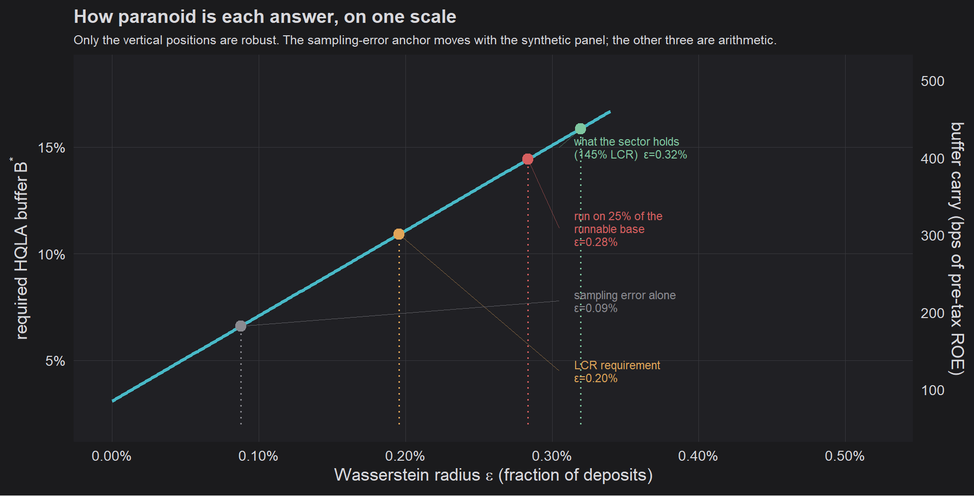
A word on units before the comparison, because two different percentages are about to appear and they measure different things. The LCR is a ratio, high-quality liquid assets divided by the thirty-day net cash outflow, and the South African minimum is 100% like everywhere else that follows Basel. Running the outflow calculation on NGFB’s book gives a denominator of 10.9% of deposits, so a bank sitting exactly on the 100% minimum holds HQLA worth 10.9% of its deposits. Surviving a run on a quarter of the runnable base takes 14.4% of deposits instead.
Both of those convert back into the ratio a treasurer actually quotes. Divide either buffer by the same 10.9% denominator and the comparison becomes a single line:
| HQLA held | as an LCR | |
|---|---|---|
| Regulatory minimum | 10.9% of deposits | 100% |
| Run on 25% of the runnable base | 14.4% of deposits | 132% |
So the minimum is short by 3.5 points of the deposit base, about R18bn on a R500bn book. Put another way, a bank complying exactly with the regulation would need to run an LCR of about 132% before its buffer covered the run this series has spent four posts isolating.
Before that gets quoted anywhere, it needs a health warning that is larger than the usual kind.
The gap depends on a bucket NGFB does not have. The LCR reserves its harshest treatment, a 100% runoff weight, for unsecured funding from other financial institutions. In South Africa that mostly means negotiable certificates of deposit sitting in money market funds. NGFB’s four-category composition, contains no such line, so the heaviest weight applied anywhere in my mapping is the 40% on non-operational wholesale. That flatters the gap, and not by a little. Carving an FI bucket out of the wholesale book closes it steadily: at 2% of the book the gap falls to 2.3 points, at 4% to 1.1 points, and at roughly 6% of the book it disappears entirely.
That is not a hypothetical range. A South African bank with an active NCD programme could easily carry an FI book of that size, and for such a bank the LCR would already require as much as the run anchor demands. So the honest statement is conditional rather than universal: for a bank whose funding looks like NGFB’s, with little or no financial-institution money, the LCR falls short of a 25% run by around three and a half points of deposits. Change the funding mix and the conclusion changes with it. This is the single largest reason to run the calculation on your own book rather than borrowing my number.
The judgement inputs move it too, though less violently. Sweeping the retail split from 40% to 70% and the term thirty-day fraction from 10% to 20% moves the gap between 2.3 and 4.9 points of deposits. The direction never changes across that grid, but the magnitude wanders by more than a factor of two.
The finding that changes the conclusion
Here is where public data does something better than confirm the model. It explains a behaviour nobody has been able to justify.
South African banks do not run at the 100% LCR minimum. The published sector aggregate (South African Reserve Bank 2023) has been around 145% for years, meaning banks voluntarily hold about half as much liquidity as the regulation demands. Everyone in treasury knows this. Nobody can defend the specific size of it. It gets justified in board packs as prudence, conservatism, or rating agency expectations, which are three ways of saying nobody has done the arithmetic. The surplus has the epistemic status of the spare wheel in the boot: universally approved of, never inspected, and widely assumed to be inflated.
Apply that ratio to NGFB’s book. A bank at 145% LCR is holding 15.9% of deposits in HQLA, against a regulatory requirement of 10.9% and a run-anchored need of 14.4%. On the ratio scale those three sit at 100%, 145% and 132% respectively, which is the whole finding in eleven characters: 100 / 132 / 145. The requirement is the smallest of the three. What banks actually hold is the largest.
The surplus covers it, with 1.4 points to spare. And unlike the gap discussed above, this comparison gets safer as you add financial-institution funding rather than more fragile, because a higher regulatory requirement lifts the observed holding too.
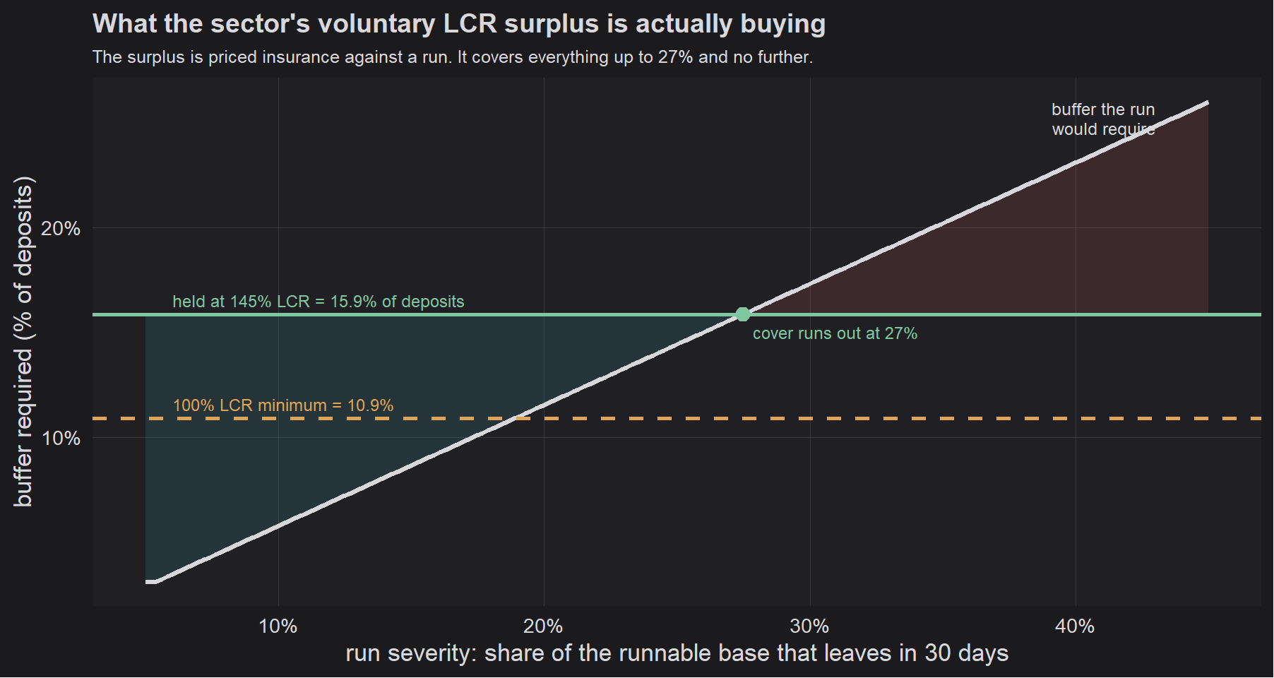
Read the green line as a coverage level. A bank holding 15.9% of deposits can absorb a run that takes up to 27% of everything capable of leaving in thirty days. Past that point the sloped line crosses over and the bank is short.
Now compare that with the assumption I fed the model. I picked a 25% run because it looked defensible against recent history. The observed surplus implies 27%.
Two numbers agreeing to within a couple of points is pleasing, and I want to be careful not to oversell it. Sweeping the judgement inputs across the same grid as before moves the implied severity between roughly 24% and 31%, and adding a financial-institution bucket pushes it higher still, towards the mid-thirties at a 6% FI book. So the honest claim is not that the industry has independently discovered my exact number. It is that the industry’s revealed behaviour and a model built from optimal transport both land in the same neighbourhood, somewhere in the region of a quarter to a third of the runnable base, having got there by completely different routes: one from a deposit book and a transport metric, the other from thirty years of South African treasurers deciding how much they could stand to lose.
That agreement is the most useful thing in this series, and it inverts the conclusion I expected to write.
The regulation is short. The banks are not. South African banks are already, in effect, running a distributionally robust buffer. They simply have no vocabulary for saying so, so the surplus gets defended as a feeling or back-of-the-envelope arithmetic rather than a scientific number.
Why this matters to a real treasury
The practical value here is not that a bank should hold more. On this evidence most large South African banks already hold roughly the right amount. The value is that a quantity currently defended with adjectives becomes a quantity defended with arithmetic, and that changes four conversations.
The surplus gets a business case. That 4.9 points of deposits held above the regulatory minimum costs about 136 bps of pre-tax ROE, roughly R618m a year on a R500bn book. Every year somebody in finance asks why the bank is carrying it, and every year treasury answers with a sentence about prudence and the question comes back. Now the answer is that it buys cover against a 27% run on the money that can actually leave, and here is the severity at which it stops working.
Cutting the buffer becomes a decision with a stated consequence. If the surplus falls from 145% to 125% LCR, the coverage level drops from a 27% run to something noticeably smaller. That is a sentence a board can vote on. “We reduced the LCR by twenty points to release capital” is not.
Risk appetite stops being an adjective. Most risk appetite statements say something like “the bank maintains a strong liquidity position.” Replace that with a run severity the bank commits to surviving, and the buffer follows arithmetically from it rather than being negotiated each year.
It gives you a like-for-like peer comparison. Two banks with different LCRs are not necessarily more or less conservative than each other, because they have different deposit mixes. Converting each to an implied run severity puts them on one axis. A bank at 130% LCR with a very sticky retail book may be covering a larger run than a bank at 160% funded by wholesale money.
What ALCO does on Monday
The dial is the deliverable. One axis is the probability that outflows breach the buffer, the other is the carry in basis points of pre-tax return on equity, using the same bridge constants I built in Post 3.
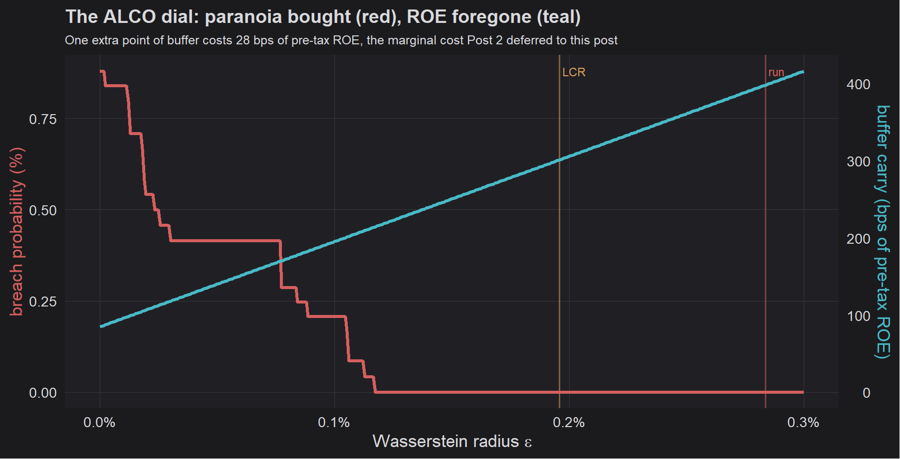
One extra point of buffer costs 28 bps of pre-tax ROE. That closes a loop opened two posts back. Post 2 scaffolded a run-fragility term in its ALCO bridge and explicitly deferred costing it to “post 4’s marginal buffer cost”, which at the time had the distinct flavour of a promissory note written by somebody with no intention of being around when it fell due. Here it is anyway. Run fragility now speaks the same language as everything else, so every point of the uninsured base you convert to insured, term out or diversify away is worth 28 basis points of ROE in buffer you never have to carry.
Three concrete uses follow. ALCO votes on a coordinate instead of adjudicating between competing apocalypses, which should shorten the meeting by approximately the length of the meeting. The gap between the regulatory and run anchors becomes a quantified statement of residual exposure rather than a vague unease that surfaces once a quarter. And the marginal cost prices funding-mix decisions directly, so a rand of uninsured wholesale money now arrives with an explicit buffer charge attached, which is a better argument for terming it out than anything currently sitting in a risk appetite statement. Most of those read as though they were drafted to be shown to somebody rather than used by somebody.
That last one deserves working through properly, because it is the lever a treasury can actually pull, and because pulling it turns out to be less obviously wise than it first looks.
The funding-mix lever, and the trap inside it
The buffer is expensive because of what sits in the runnable base. So the obvious move is to shrink that base: take uninsured wholesale money that can leave inside thirty days and push it out beyond thirty days, where the LCR stops counting it and a thirty-day run cannot reach it.
The mistake is to stop the analysis there. Terming out funding is not free. Depositors and wholesale counterparties charge you for the privilege of not being able to leave, and on a curve as steep as South Africa’s that term premium is substantial. If you show only the buffer saving and not the funding cost, you have invented a free lunch, which is precisely the thing this blog exists to be rude about.
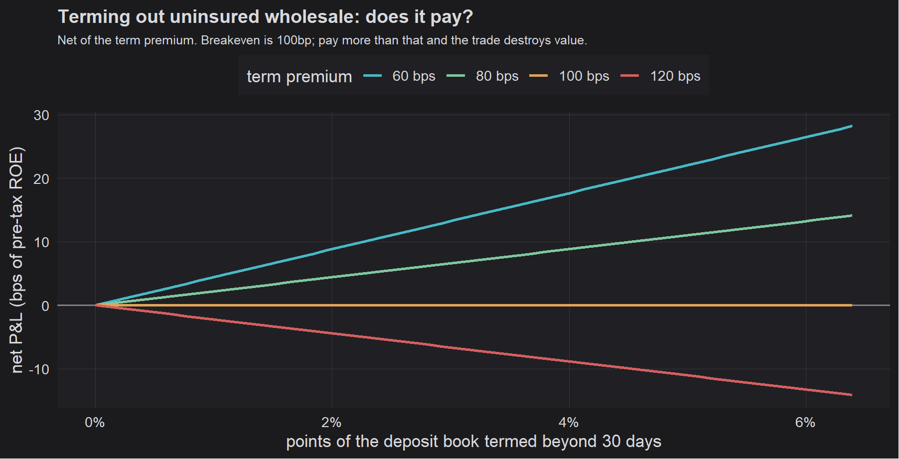
The breakeven term premium is 100 basis points, and it is worth seeing where that comes from, because it is simpler than the chart suggests.
Move one point of the deposit base out beyond thirty days. The LCR requirement falls by that point multiplied by the bucket’s runoff weight, so you release $0.40$ of a point of HQLA. Each point of HQLA released earns the redeployment spread instead of the repo rate, which is worth $2.5\%$. So the saving is $0.40 \times 2.5\% = 1.0\%$ of the point you moved. The cost is the term premium on that same point. Setting them equal:
$$\text{breakeven term premium} \;=\; \text{runoff weight} \times \text{HQLA give-up spread}.$$Every other quantity cancels. The balance sheet size, the leverage, the equity base, the deposit mix: none of them appear. For non-operational wholesale at a 40% weight and a 250bp spread, the answer is 100bp and it would be 100bp at any bank. The same rule prices every other bucket: operational wholesale at 25% breaks even at 63bp, less-stable retail at 10% at just 25bp. That is a hurdle rate a funding desk can carry in its head.
That single number is worth more to a treasurer than most of the machinery above it, because it converts a permanent argument into a price test. The question stops being “should we term out more of the wholesale book” and becomes “can we do it inside a hundred basis points”, which a funding desk can answer in an afternoon.
Two practical limits. The lever is small, because non-operational wholesale is only 6.4 points of NGFB’s book, so terming out every last rand of it releases about R13bn of HQLA and 14 bps of ROE at an 80bp premium. And the payoff is linear in the premium, so the whole case lives or dies on a number that moves with the curve.
The trap
Now look at what terming out does to the two buffers at the same time.
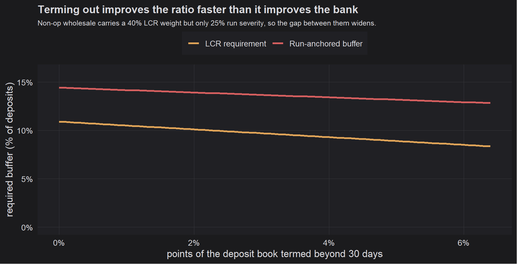
Both lines fall, which is good: terming out genuinely reduces risk as well as the requirement. But they fall at different speeds. Term out the whole non-operational wholesale book and the LCR requirement drops from 10.9% to 8.4% of deposits, while the run-anchored buffer only falls from 14.4% to 12.8%. The gap between them widens, from 3.5 to 4.5 points of deposits.
The mechanism is simple once you see it, and it has a one-line proof. Term out $s$ points of a bucket whose runoff weight is $\rho$. The LCR requirement falls by $\rho s$. The runnable base falls by $s$, so the run-anchored buffer falls by $\kappa s$. The gap between them therefore changes by
$$\frac{\mathrm{d}(\text{gap})}{\mathrm{d}s} \;=\; \rho - \kappa.$$The gap widens whenever the bucket’s regulatory runoff weight exceeds the run severity you actually believe in. For non-operational wholesale that is $40\%$ against $25\%$, so every point termed out widens the gap by $0.15$ of a point. You are improving the metric faster than you are improving the bank. The effect reverses only if you think a run would take more than 40% of that funding, at which point the LCR weight is no longer generous but stingy.
This also tells you which buckets are safe to optimise. Any bucket whose runoff weight sits below your assumed run severity gives you more real risk reduction than regulatory credit, and terming those out is unambiguously honest. Stable retail at 5% and less-stable retail at 10% are both far below a 25% run assumption. It is precisely the buckets the LCR punishes hardest that reward gaming.
This is not an argument against terming out, which remains sensible at the right price. It is an argument against using the LCR as your scoreboard while you do it. Optimising the ratio instead of the risk is the funding-book version of driving to the Gautrain station to beat the traffic and then spending twenty minutes hunting for parking. A treasury optimising purely to the ratio will work through the funding book in order of runoff weight, which is the order in which the regulation over-rewards the action rather than the order in which risk is actually reduced. The published research on South African banks already shows exactly this behaviour. Mabandla and Marozva (2026) find, on a 2015–2024 panel of the leading local banks, a significantly positive association between the LCR and both total and long-term debt ratios, and a negative one with short-term debt. The parallel NSFR evidence points the same way (South African Reserve Bank 2024b; Basel Committee on Banking Supervision 2014). Some of that is genuine prudence. Some of it, on this analysis, is the ratio paying a premium for a particular trade.
The practical fix costs nothing. Run both measures side by side. If a funding action improves the LCR much faster than it moves the run-anchored buffer, that is a signal to check whether you are buying risk reduction or buying optics.
The series, in one currency
In every post I hoped to convert the findings into basis points of NIM converted to ROE. All four now do. What they do not do is add up, and the reason for that is worth more than a total would be.
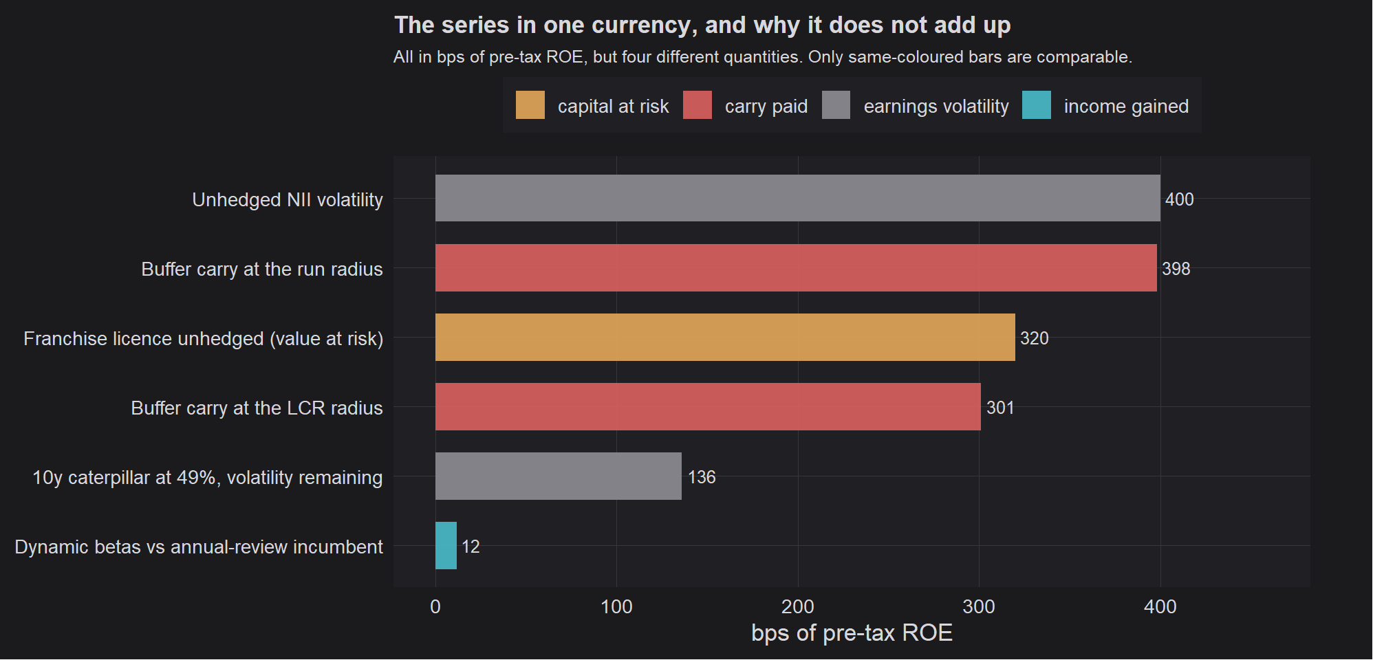
Post 1’s 12 bps is income gained, a real and recurring improvement from modelling deposit betas dynamically instead of resetting them each January with roughly the conviction of a gym contract. Post 3’s figures are earnings volatility rather than income: a ten-year caterpillar at a 49% hedge ratio takes year-on-year NII volatility from 400 bps of ROE down to 136. Post 2’s is capital at risk under a ±200bp shock. Post 4’s are carry paid, meaning money genuinely handed over every year in exchange for surviving something that has not happened yet.
Add those together and you get a large number that means absolutely nothing. A basis point of recurring income, a basis point of volatility, a basis point of stressed capital and a basis point of paid carry are four different animals wearing the same uniform. Treasury reporting does this all the time, and the resulting totals enjoy the considerable advantage of being impossible for anyone to check. It is the balance-sheet cousin of an SOE annual report, in which every number is individually defensible and the sum has never met any of them.
What the chart does support is comparison within colours, and the two red bars are where to look. The distance between them - the LCR buffer against the run buffer - is roughly 97 bps of pre-tax ROE. That is the annual price of the gap between what the regulation asks for and what a serious run would demand, and the sector is already paying it voluntarily without calling it that.
What didn’t work and some health warnings
The standing rule holds, and this post has rather more to declare than most.
Two specification traps sit in the middle of this method, and both are silent. The first is the $\tfrac{1}{1-\alpha}$ in the boxed formula: a CVaR constraint is not an expectation constraint, and treating it as one understates the radius by a factor of 40 without anything visibly breaking. The second is the runnable base, where counting all uninsured deposits rather than only the uninsured money available inside thirty days overstates the run anchor by about two and a half times. Neither error announces itself. Both produce a perfectly plausible-looking number, which is exactly what makes them worth naming.
Retail stability is calibrated in, not discovered. The category volatilities in the synthetic panel are ordered to match the LCR runoff weights, so naturally the attribution reports that retail is sticky and wholesale is flighty. That is the calibration admiring itself in a mirror. What is not circular is the composition, the betas, the CODI coverage and the bridge constants, all of which are real series outputs and all of which drive the headline. The synthetic panel moves the CVaR at the centre of the ball. It does not touch the run anchor, which is arithmetic on public numbers. The punchline surviving the synthetic layer entirely is the only reason this is worth publishing.
BA 900 carries no stable/less-stable tag. That classification lives in the supervisory BA 325 return, which stays behind the curtain. The retail/wholesale split and the term within-30-day fraction above are judgement rather than measurement, and they move the regulatory NCO materially. A real implementation would pull them from the bank’s own book, where they are simply known, which does rather undercut the pretence that any of this is reproducible from public data alone.
The radius does two jobs and I have spent this whole post calling it one dial. It is at once a confidence region for sampling error and a correction for structurally unobservable gross flow - two different things wearing one coat. Those are different species of ignorance and they should not really be sharing a parameter. Presenting three anchors is an attempt at honesty about the problem rather than a fix for it. A cleaner treatment would separate them and I do not have one.
The net-versus-gross problem is still not solved. It has been reframed from something you measure into something you price, which counts as progress of a sort, but the underlying limitation has bound every post in this series and it binds this one too. Customer-level data would break it in an afternoon. Customer-level data is precisely what I am not allowed to publish.
The breach curve validates in-sample. The dial’s probabilities are computed against the same pooled sample that produced the CVaR, which is the oldest trick in the backtesting book and one this series has fallen for before. The finite-sample bound in Mohajerin Esfahani and Kuhn (2018) is the reason to trust the method. The in-sample curve should not be mistaken for a survival guarantee. Rolling-origin validation is the obvious next step and it is not done here because, believe it or not, I do have a life.
The ICC is estimated from five banks. A 4.9% intraclass correlation off five groups carries a confidence interval you could comfortably drive a Hilux bakkie through. Agreeing with Post 1 is encouraging. Agreeing to within a percentage point is luck, and I am not going to pretend otherwise.
The panel is calibrated to a monthly standard deviation of 0.87%, deliberately at the calm end of plausible. That choice drives the empirical CVaR and therefore the sampling anchor, and it drives nothing else: the LCR requirement, the run-anchored buffer, the sector comparison and every funding-mix result are pure arithmetic on the composition and the runoff weights. Which is fortunate, because the sampling anchor is the one number here that a determined person could talk me into moving.
The term bucket uses a retail-like runoff weight. Term deposits maturing inside thirty days get 10% in my mapping, which is roughly right for retail term money and too gentle for wholesale term money. Since term is 40% of the book, this assumption is load-bearing, and a real implementation would split it by counterparty rather than applying one blended rate.
The run anchor assumes CODI-insured money cannot run at all. It can. Basel assigns insured stable retail a 5% runoff weight rather than zero, precisely because insurance dampens a panic without abolishing it. Treating the insured bucket as entirely locked shrinks my runnable base and therefore understates the run-anchored buffer. Letting insured deposits run at a fifth of the rate uninsured ones do lifts the buffer from 14.4% to about 14.6% and widens the gap by roughly two tenths of a point. The effect is small only because the insured bucket is about 8% of NGFB’s book, and it runs in the conservative direction, so the published gap is if anything a floor on this axis.
Everything scales linearly in the run severity. The run anchor is a quarter of the runnable base because I chose a quarter. Pick 20% and the anchor drops below what the sector holds by a comfortable margin; pick 30% and the surplus stops covering it. The agreement between my 25% and the 27% implied by the observed surplus is genuinely reassuring, but it is one number agreeing with one number, and I chose mine first.
The sector LCR is a dated aggregate. The 145% figure is a published sector-level number from 2022, and the SARB itself notes that a high average masks bank-specific dynamics. Using the aggregate is deliberate, since it is the only version of this comparison that identifies nobody, but a current figure would be better and an individual bank’s own ratio would be better still. Anyone running this internally should use their own.
Constant deposit growth is still wrong. Post 3 measured BA100 core deposit growth at 8.07% a year and found it correlates +0.62 with the repo level. The panel here uses a constant drift, the same simplification Post 3 documented and declined to patch. In a cutting cycle the drift and the stress turn up together, and nothing in this model has any idea that happens.
The end of the series
Four posts, one synthetic bank, and a conclusion that got there via the R62.
South African deposits turn out to be remarkably well behaved. They do not run off. They do not chase rates at any speed the data can detect. They do not differ much from one large bank to the next. Every sophisticated technique I threw at the smooth part of the problem, from state-space filtering to simulation-differentiated duration to spectral filter design, confirmed that the smooth part of the problem is small. The optimiser in Post 3 improved on the industry-standard hedge by exactly nothing, which remains my favourite result in the whole series precisely because of how spectacularly unhelpful it is. Somewhere a vendor is selling that same optimiser with a licence fee attached.
The nulls were not the whole harvest, though, and it would be false modesty to pretend otherwise. Along the way the series produced a defensible set of product-level betas, a franchise licence of 5.12 years that quantifies what the deposit book is actually worth as funding, a hedge ratio of 49% that follows from the betas instead of from an argument, a 62% cut in earnings volatility for running it, and 12 basis points a year for the simple act of not treating deposit pricing as an annual event. None of that is glamorous. All of it is bankable, which glamour rarely is. What is far more valuable than the results is the methodology.
What is left is the discontinuity. The run does not appear in the returns, cannot be estimated from them, and will not be modelled into submission by anybody working from public data. The only move available is the one this post makes: stop pretending to estimate it and price it instead.
And then the useful thing happened, which I did not plan and cannot take credit for. Having built an apparatus to price a run, I pointed it at what South African banks already do and found they have been pricing one all along. The 145% sector LCR, that stubborn surplus nobody can quite defend in a board pack, turns out to be cover against a 27% run on the money that can actually leave. The regulation asks for 100%, the run needs 132%, and the industry settled on 145% without ever writing down why. The optimal transport did not tell the industry to do anything different. It told the industry what it had already decided, in language it can now use.
That is a smaller claim than the one I set out to make and a more useful one. Most quantitative work in this field either confirms what practitioners knew or contradicts it badly enough to be ignored. Occasionally something lands in the middle: it agrees with the practitioners and hands them the argument they were missing. The radius of a Wasserstein ball is an odd thing to bring to an ALCO, but it says the one thing a liquidity buffer has never been able to say for itself. This is how wrong we are prepared to be, and this is the annual invoice.
This ran on a bank that does not exist, so I cannot tell you what it would do to yours. What I can say is that the spread of outcomes is unusually narrow. At best it is worth real money. More than a dozen basis points of ROE a year for pricing deposits dynamically, and a hundred-basis-point hurdle rate for funding decisions that are currently argued rather than costed. At worst, nothing on the balance sheet changes and ALCO simply gets a defensible number where it has been using an adjective. For quantitative work, that is an unusually high floor.
Sold voetstoots, as the offer to purchase has it: none of this is advice, and the buffer at your own bank should be sized by people with access to the BA 325.
References
Artzner, Philippe, Freddy Delbaen, Jean-Marc Eber, and David Heath. 1999. “Coherent Measures of Risk.” Mathematical Finance 9 (3): 203–28. https://doi.org/10.1111/1467-9965.00068.
Basel Committee on Banking Supervision. 2013. Basel III: The Liquidity Coverage Ratio and Liquidity Risk Monitoring Tools. Bank for International Settlements. https://www.bis.org/publ/bcbs238.htm.
Basel Committee on Banking Supervision. 2014. Basel III: The Net Stable Funding Ratio. Bank for International Settlements. https://www.bis.org/bcbs/publ/d295.htm.
Blanchet, Jose, and Karthyek Murthy. 2019. “Quantifying Distributional Model Risk via Optimal Transport.” Mathematics of Operations Research 44 (2): 565–600. https://doi.org/10.1287/moor.2018.0936.
Diamond, Douglas W., and Philip H. Dybvig. 1983. “Bank Runs, Deposit Insurance, and Liquidity.” Journal of Political Economy 91 (3): 401–19. https://doi.org/10.1086/261155.
Drechsler, Itamar, Alexi Savov, and Philipp Schnabl. 2021. “Banking on Deposits: Maturity Transformation Without Interest Rate Risk.” The Journal of Finance 76 (3): 1091–143. https://doi.org/10.1111/jofi.13013.
Fournier, Nicolas, and Arnaud Guillin. 2015. “On the Rate of Convergence in Wasserstein Distance of the Empirical Measure.” Probability Theory and Related Fields 162 (3–4): 707–38. https://doi.org/10.1007/s00440-014-0583-7.
Gao, Rui, and Anton J. Kleywegt. 2023. “Distributionally Robust Stochastic Optimization with Wasserstein Distance.” Mathematics of Operations Research 48 (2): 603–55. https://doi.org/10.1287/moor.2022.1275.
Mabandla, Ndonwabile Zimasa, and Godfrey Marozva. 2026. “The Effect of Regulatory Liquidity Measure on Bank Capital Structure: Evidence from South Africa.” Risks 14 (5): 109. https://doi.org/10.3390/risks14050109.
Mohajerin Esfahani, Peyman, and Daniel Kuhn. 2018. “Data-Driven Distributionally Robust Optimization Using the Wasserstein Metric: Performance Guarantees and Tractable Reformulations.” Mathematical Programming 171 (1–2): 115–66. https://doi.org/10.1007/s10107-017-1172-1.
Motau, Terry. 2018. VBS Mutual Bank: The Great Bank Heist. Investigator’s Report to the Prudential Authority. South African Reserve Bank, Prudential Authority.
Rockafellar, R. Tyrrell, and Stanislav Uryasev. 2000. “Optimization of Conditional Value-at-Risk.” Journal of Risk 2 (3): 21–41. https://doi.org/10.21314/JOR.2000.038.
Rockafellar, R. Tyrrell, and Stanislav Uryasev. 2002. “Conditional Value-at-Risk for General Loss Distributions.” Journal of Banking & Finance 26 (7): 1443–71. https://doi.org/10.1016/S0378-4266(02)00271-6.
South African Reserve Bank. 2023. Financial Stability Review. South African Reserve Bank. https://www.resbank.co.za/en/home/publications/Reviews/financial-stability-review.
South African Reserve Bank. 2024a. Corporation for Deposit Insurance: Deposit Insurance Scheme for South Africa. Corporation for Deposit Insurance, operational 1 April 2024. https://www.resbank.co.za/en/home/what-we-do/Deposit-Insurance.
South African Reserve Bank. 2024b. The Impact of Liquidity on Bank Lending in South Africa. Working Paper WP/24/10. South African Reserve Bank. https://www.resbank.co.za/en/home/publications/publication-detail-pages/working-papers/2024/the-impact-of-liquidity-on-bank-lending-in-south-africa.
South African Reserve Bank. 2025. BA 900: Institutional and Maturity Breakdown of Liabilities and Assets (Monthly Economic Returns of Banks). Prudential Authority, selected SA banks data. https://www.resbank.co.za/en/home/what-we-do/statistics.
Villani, Cédric. 2009. Optimal Transport: Old and New. Vol. 338. Grundlehren Der Mathematischen Wissenschaften. Springer. https://doi.org/10.1007/978-3-540-71050-9.